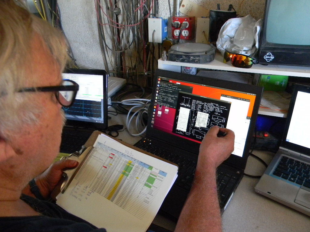
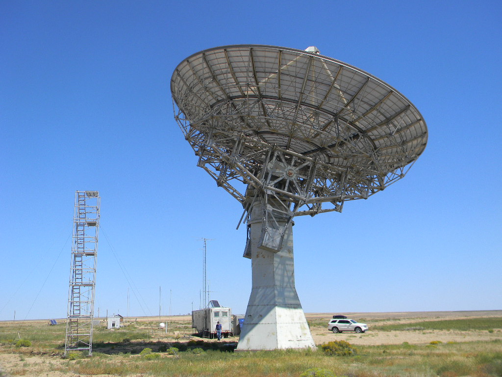
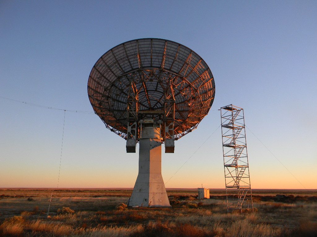
Glenn Davis and Dan Layne made observations for pulsars at our Haswell antenna site this week, on Tuesday November 1, 2022. They successfully observed for the first time pulsar B1556 -44, making this the 23rd pulsar DSES has observed to date.
The PDF files in this post are their observation and data report, and an updated list of pulsars detected by DSES to date.
Text and photos by Gary Agranat. Analysis pdf by Rich Russel.
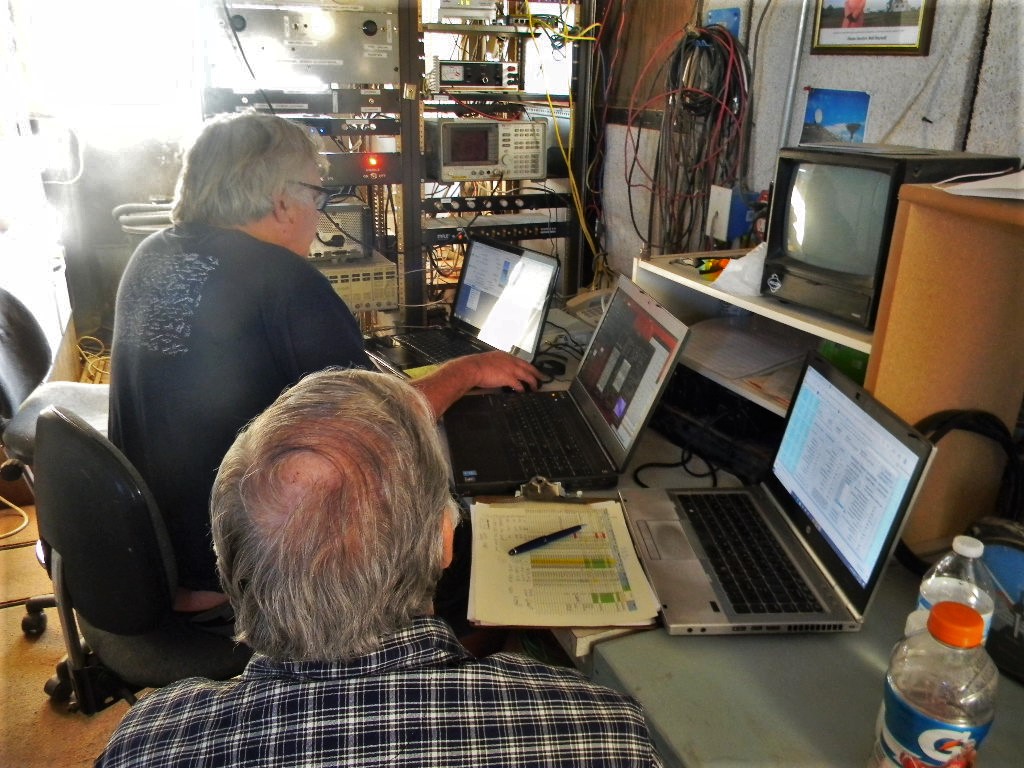
On Saturday September 12, 2020 an observing team of Rich Russel, Bob Haggart, Bill Miller, and Gary Agranat spent the day observing pulsars. This is the first observing session since we recalibrated the 60-foot antenna azimuth pointing the weekend before. The team observed 3 pulsars we had not seen before. Plus several other pulsars were attempted. The team spent the whole day at the site, from about 9 AM to 7 PM.
The pulsar signals are so faint that we cannot detect them directly. To observe them, we have to point to the correct celestial coordinates and then track that point as the Earth rotates. While we are pointed, our computer accumulates the signal data. We need at least a half hour continuously tracking the position. At this session some of our observing runs lasted 2 hours, for the fainter objects. At previous sessions we have tracked for as long as 4 hours.
After the observing track, we have our software process the data. The random background noise should cancel itself out. But the pulse signals should build up with time. If we have the correct timing interval of the pulses, and if everything else is working, the computer display will show the pulses, and several other parameters.
Pulsars are very unusual objects. These are what remain of massive stars (greater than 5 solar masses) after they use up all their fuel for nuclear burning. These more massive stars fuse heavier and heavier elements at their cores until they start to fuse iron from silicon. Unlike the fusion of other elements, iron requires energy to fuse, rather than produce energy. The sudden reduction of energy at the core drops the temperature and pressure there. The pressure at the core is no longer enough to counter the weight of the star’s material above it. Gravity is now the stronger force, and the material above collapses in on the center. The pressure and temperature at the core then becomes even higher, which starts new reactions that fuse the matter at the center to neutrons, and and which also generates neutrinos. The outer layers falling in at great speed bounces back out. The result is a supernova explosion. What remains is the neutron star at the center. It is extremely massive and compact. And like an ice skater rotating faster as the arms are brought in, the star’s rotation speeds up immensely. The star’s magnetic field also has become compressed and much more intense. Charged particles will rotate around the magnetic field lines, with very high energy. Whenever charged particles are forced to deviate their paths from a straight line they emit electromagnetic energy, like visible light and radio. At the neutron star’s poles, this energy is channeled out, with immense energy. Because the magnetic poles are generally not at the same spots as the rotational poles, the beam of this light and radio is spun around like a light house. If Earth happens to be in the path of such a beam, we detect that as a pulsar. So that’s what we’re observing. These neutron stars are hundreds and thousands of light years away.
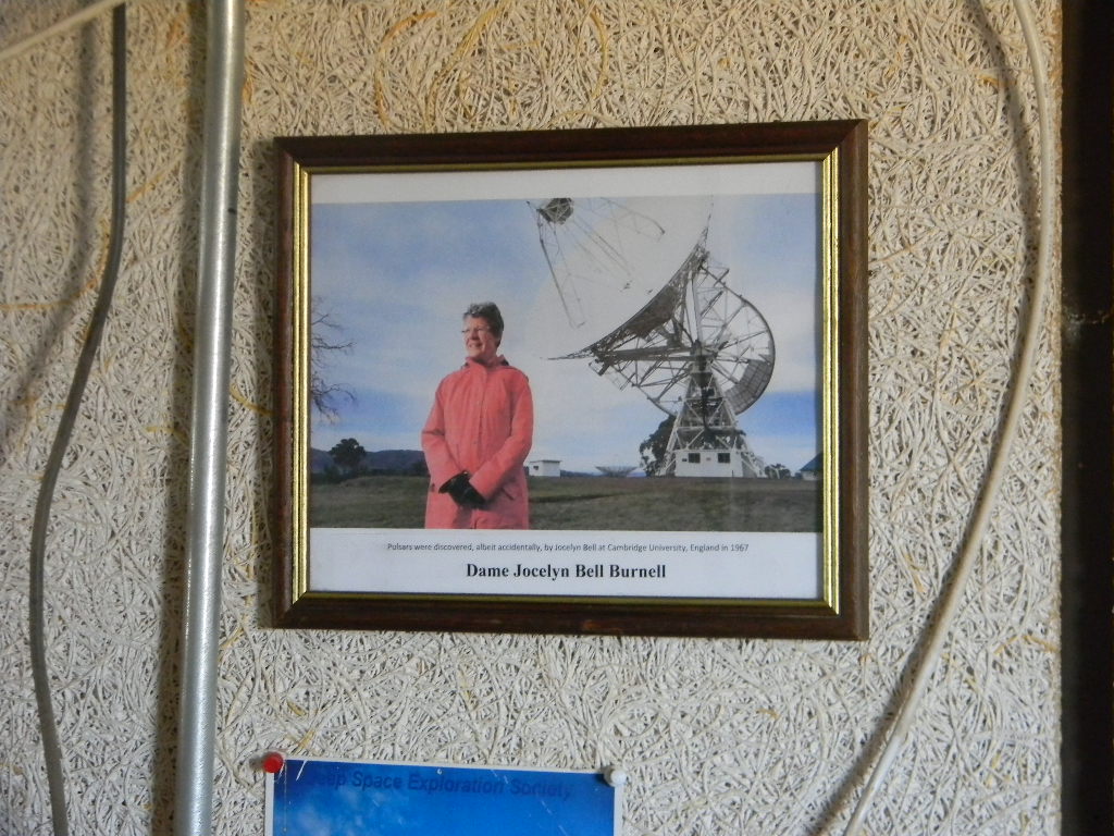
Pulsars were first discovered by accident in 1967, by Jocelyn Bell (now Jocelyn Bell Burnell) who was then a graduate student at Cambridge University. Bob contributed a recent photograph of her, posed by some radio telescopes. We now proudly have that displayed on the wall above our computer displays.
Because the observing runs take a while, for this session we decided to try watching some videos. Bob brought a DVD player and a large monitor. Gary brought some educational videos, including one about the Crab Nebula and pulsars. Rich brought some movies.
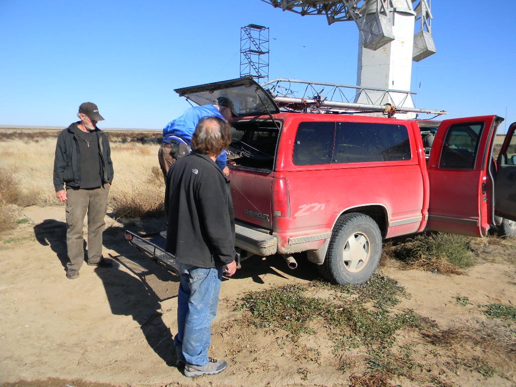
On this work trip the team also inspected damage to our ham radio antennas, damage probably from the storm weather over the past months. 7 radials at the base of the vertical antenna were damaged. And the 3 element Yagi antenna on tower was slightly tilted along its longitudinal boom.
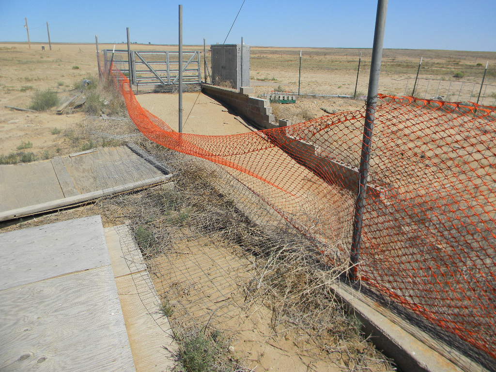
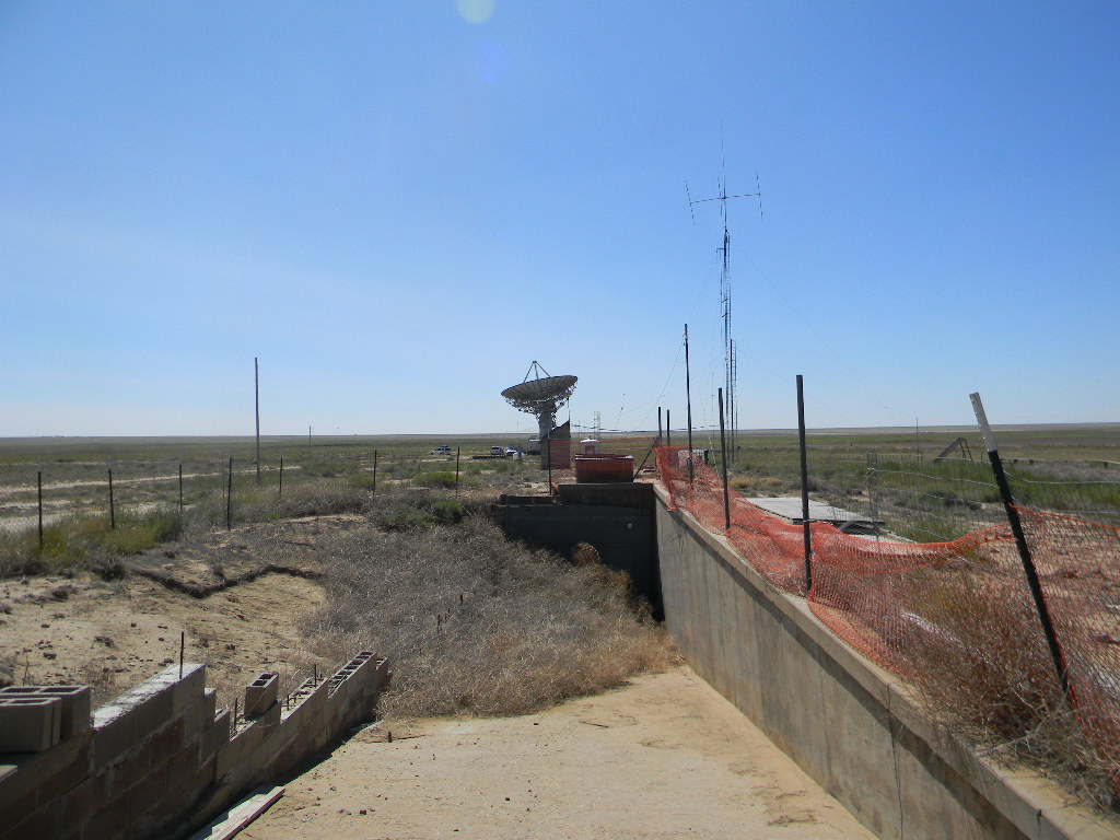
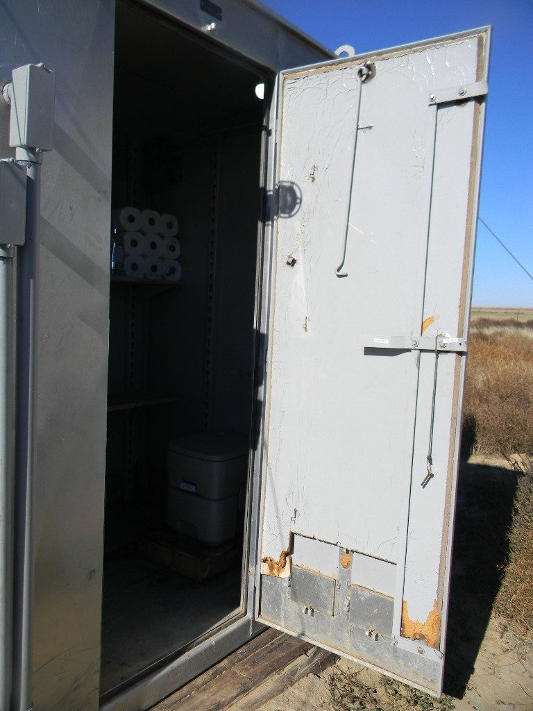
Tumbleweeds also had accumulated again at the bunker ramp. Some of the surrounding fence had also been damaged from the weather. Rich Russel brought some fencing to use in the future, to place over the immediate entrance path to the bunker door.
Repair of the ham antennas and ramp clearing will be planned for a future work trip.
Below is a photo narrative of the day’s work.
It was an excellent day’s work.
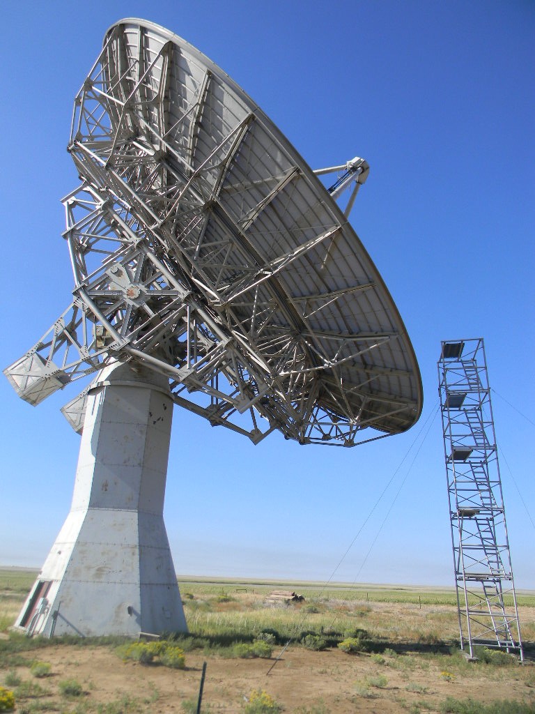
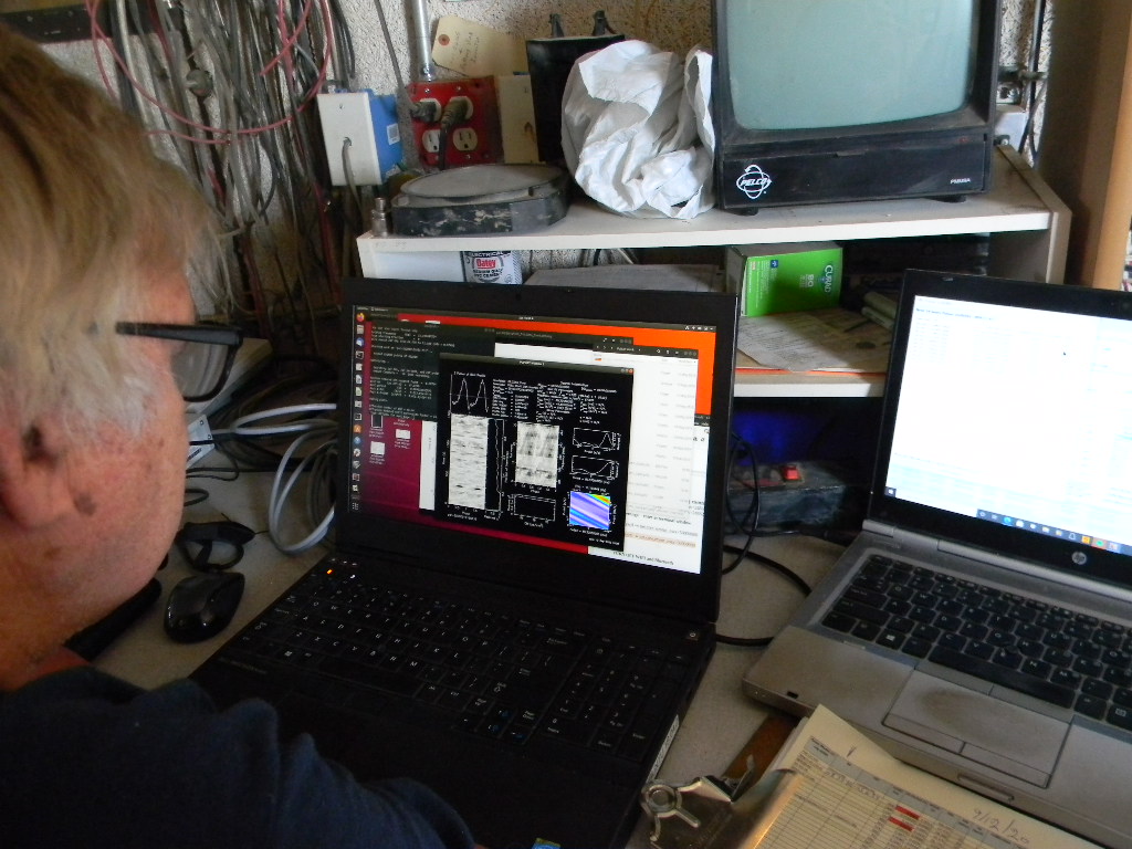
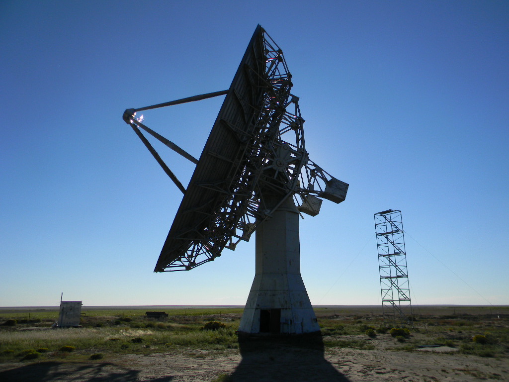
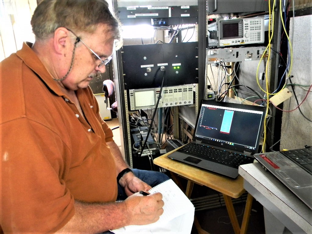
At the start of observations, we point to and observe a pulsar with a strong signal that we know we should be able to reliably receive and analyze. If we cannot detect it, that indicates something is wrong with our system. We would then troubleshoot rather than waste our time trying to observe. Here the antenna is pointing to a pulsar we use as a reference source, B0329+54. It is located in the circumpolar sky to our north, so it is always visible above the horizon for us.Bill Miller, Rich Russel, and Bob Haggart starting observations in the Operations Trailer.After we checked our equipment and processes, we tried looking for some pulsars that were relatively low on the horizon to our south. Objects that appear to the south are above the horizon only briefly. They rise in the southeast, as the Earth turns they continue to rise in a shallow arc above the southern horizon, then soon set in the south west. If we want to try to observe them, we have just a short window of time to find and track them. Being low on the horizon adds some bias errors and attenuation to the observations. At this session we didn’t succeed in observing any pulsars that were close to the southern horizon.On this run, the display shows we did not get good data. The software is attempting to synchronize our data with an expected pulse period. In the top window display that is open, for good data we would expect to see clearly spiked peaks rising from a lower noise floor. And in the white rectangular box below that, we would expect to see a signal at that timing accumulate under such spikes. There is no pattern of periodic data. The white box to the right shows timing at the bottom with radio frequency at the side (going up). Because the pulsar signal is broad band (it is spread broadly over a wide range of frequencies), we would expect to see a continuous line of signal from bottom to top, across the frequencies. But we do not see that. (You can click this image to enlarge it.)
The two graphs in the center right tell us we don’t have a definitive measure of a pulse rate, and a steady change in pulse rate. The pulsars are generally slowing down with time, at a very slow but measurable pace. The display is showing the algorithms cannot fit a pattern. If it could, the two peaks would both be centered.Our Operations Trailer
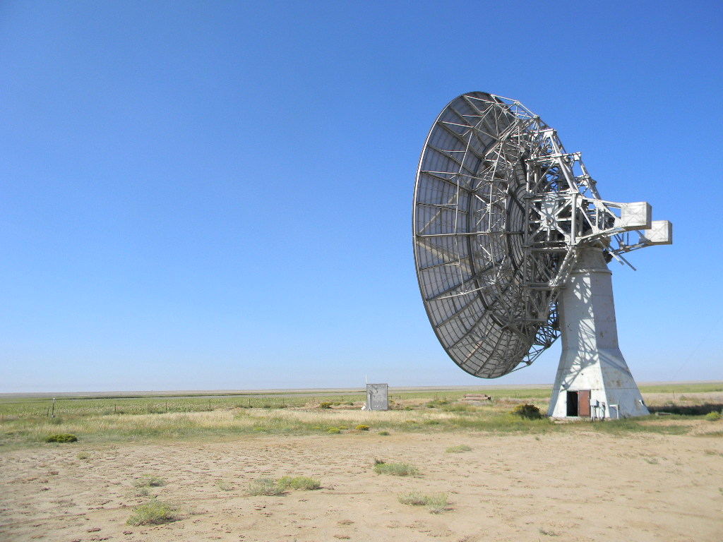
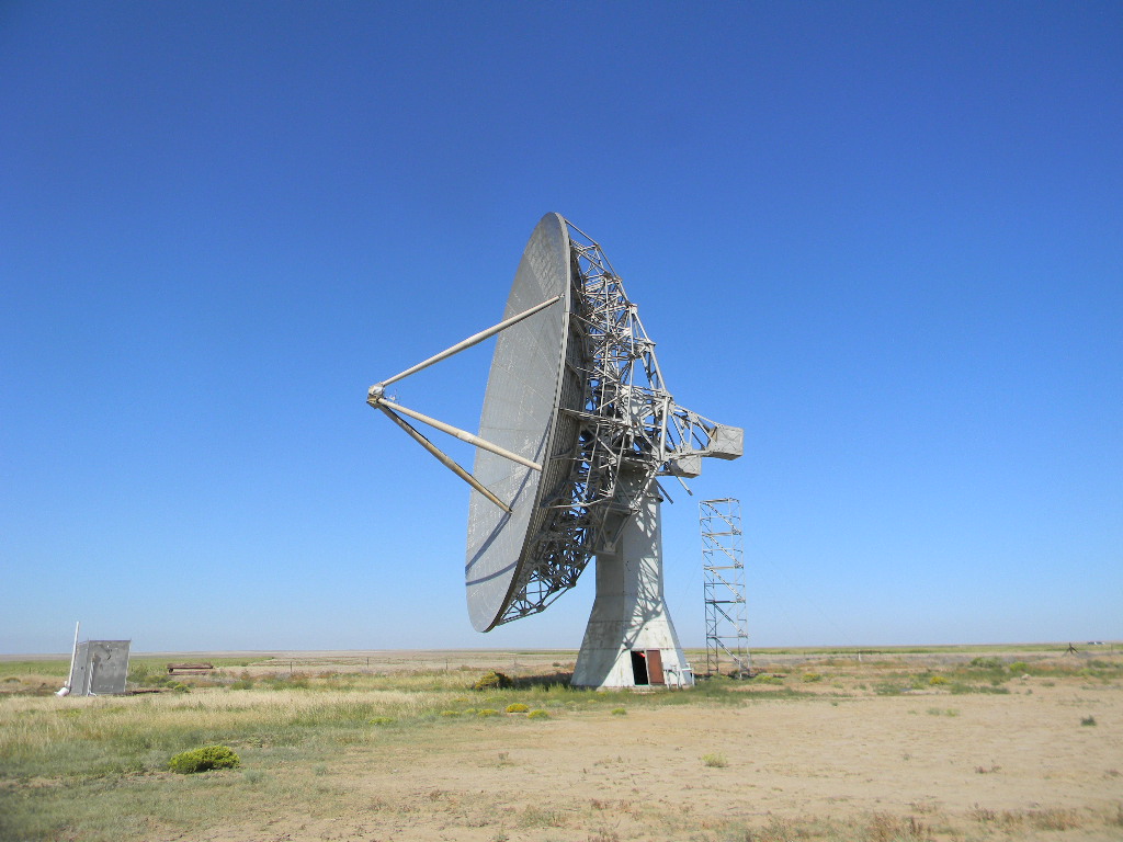
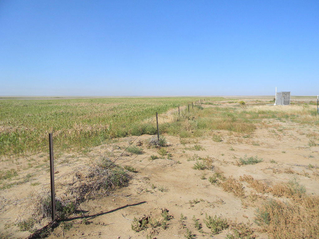
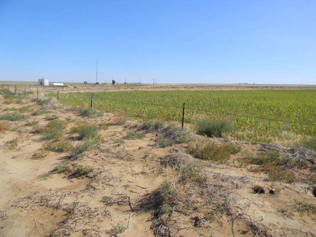
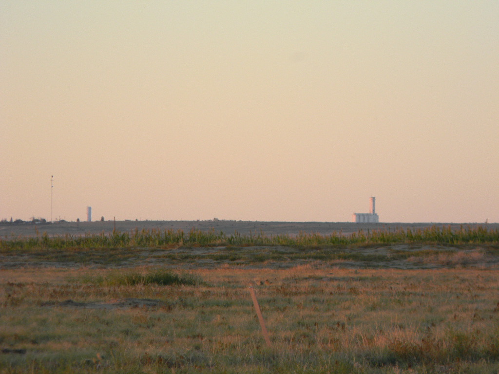
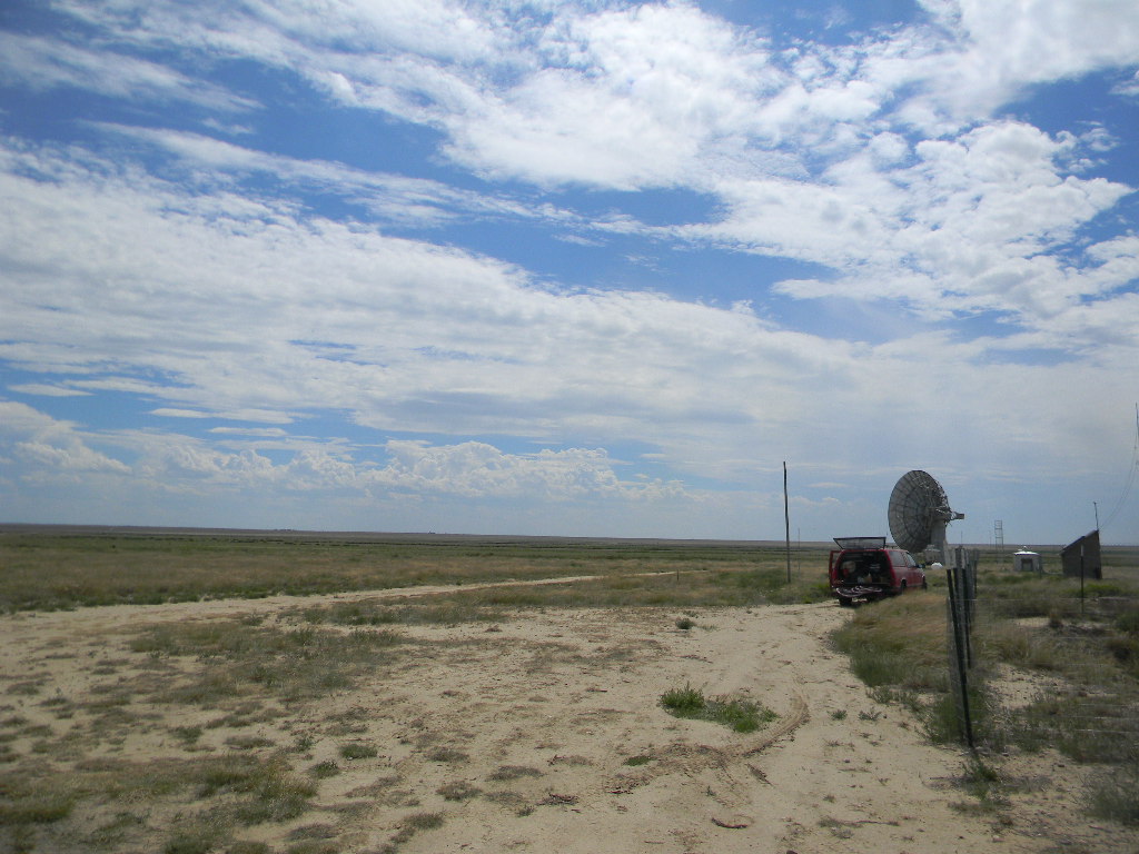
Our antenna site is surrounded by farm fields.
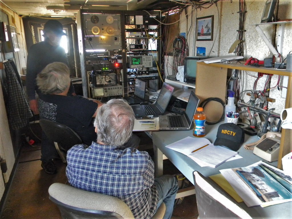
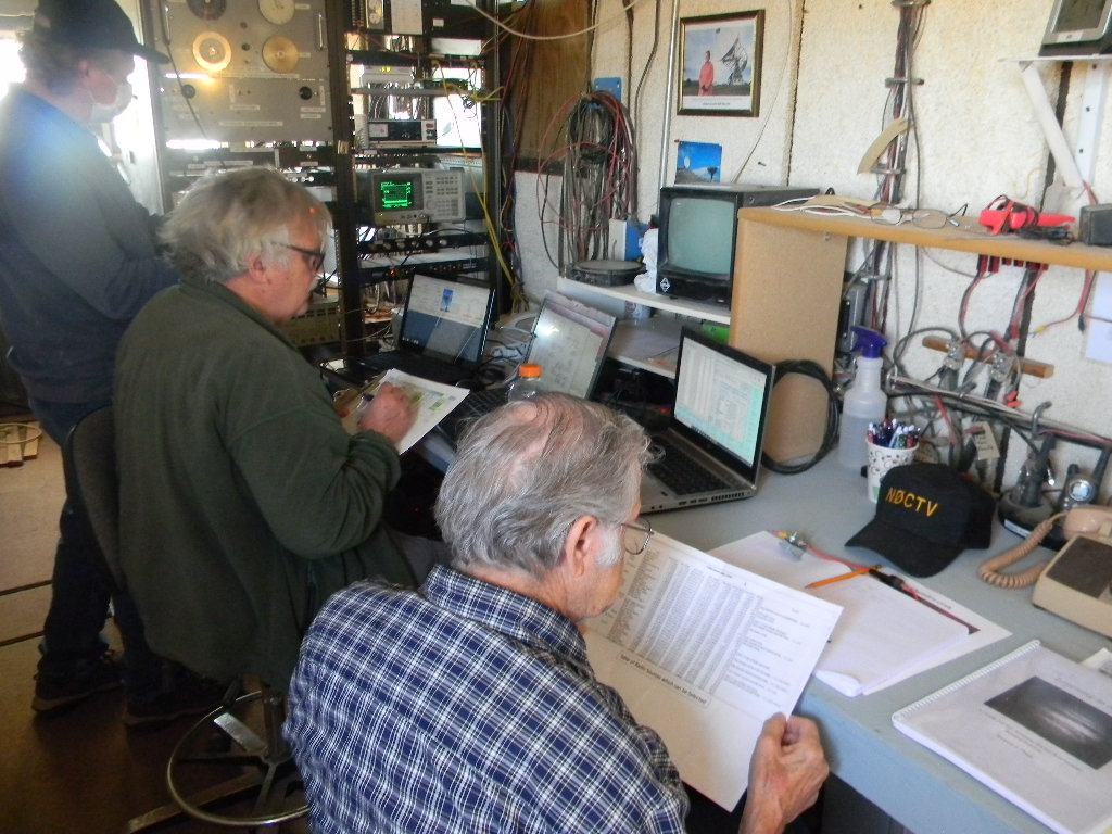
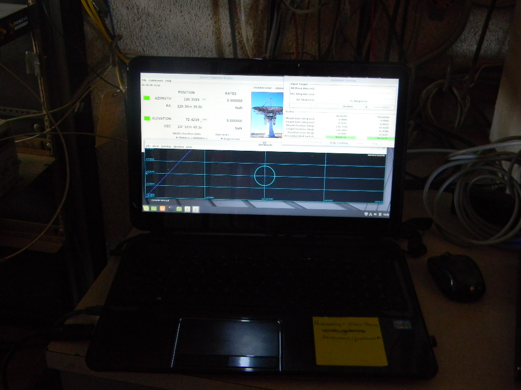
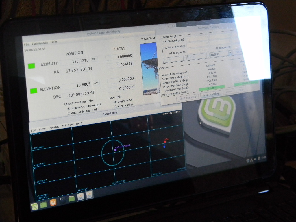
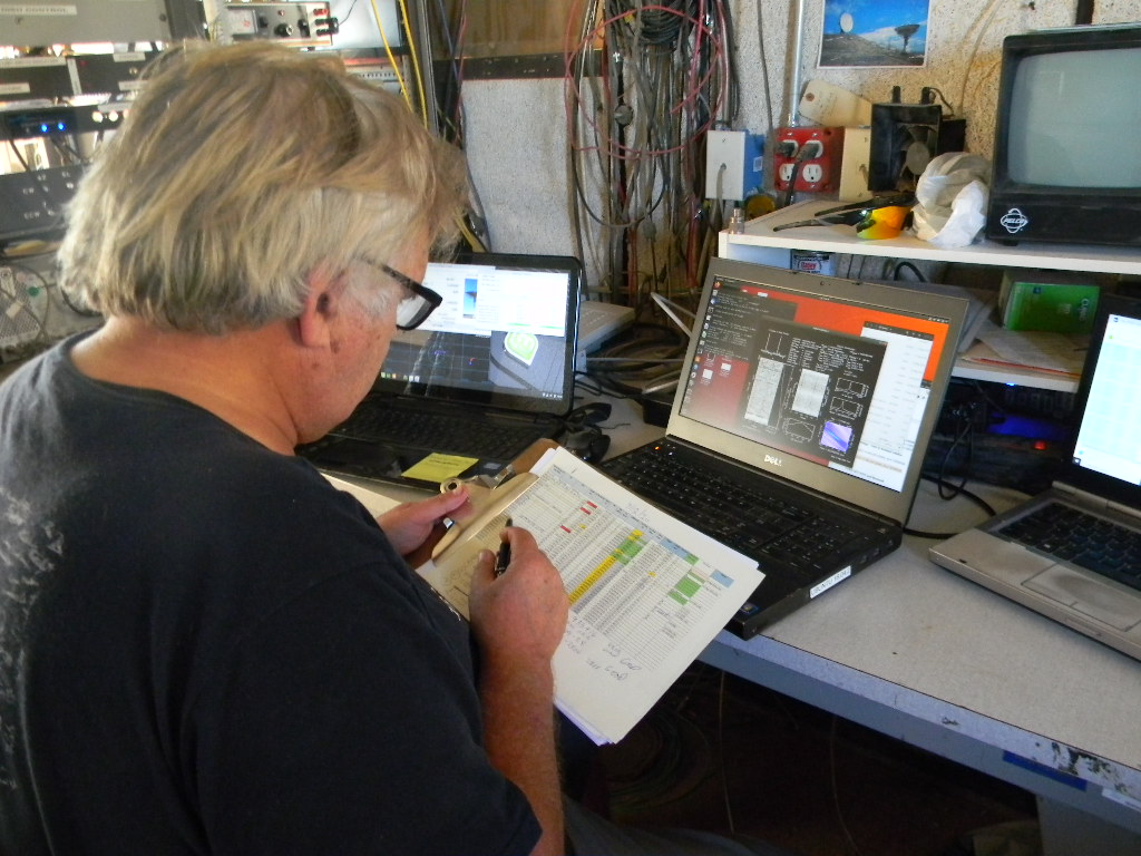
Rich and Bob are checking data for each next pulsar we attempt to observe. Besides the celestial coordinates, we need to know the expected energy flux. If the signal is weaker, we need to observe and track on the object for a longer period of time. We also need to know the expected pulse timing and several other parameters.We have up in our control room a framed photo of Jocelyn Bell Burnell, contributed by Bob Haggart. She discovered pulsars serendipitously while she was a graduate student at Cambridge University in 1967. Rich is assessing a good data set we just got. Here you can see the distinctive pulse timing spikes in the upper left. In the center white plot, you see two straight lines, representing the pulsed signal, across the spectrum of frequencies we observed (we observe across a bandwidth of 10 MHz). At the right, the software found a good analysis for the rate and change of rate of the pulses. The bottom plot slopes downward slightly to the right. That is showing us the dispersion of the signal, something we expect to see. As the pulsar radio signal travels through interstellar space, it has to go through dust and magnetic fields. The effect is that the longer the radio wavelength, the slower the signal will propagate through space. Therefore the longer wavelength signal will arrive slightly later than the shorter. This is an indirect measure of the distance to the pulsar. If the algorithm was just trying to make sense of random noise, we would not see this result in our data. (You can click this image to enlarge it.)This is a close-up of our SYSTEM 1 software display for pointing our dish antenna. The antenna now can be pointed manually or with several levels of automation.
The first accomplishment was to translate the actual azimuth and elevation pointing angles of the antenna through encoders with digital readouts. That azimuth and elevation angles were then correlated with the celestial coordinates at the given time. That required a good timing reference, as well as an accurate fix on our longitude and latitude. We now take care of that timing and position fix with GPS.
The upper part of the screen shows the direction the antenna is aimed at, in both azimuth and elevation angles, and the celestial coordinates of Right Ascension (RA) and Declination. There is more on the right side that was added later which I will discuss shortly.
The next development was to have a visual reference of the celestial sky, with its coordinate grid system and celestial objects we are interested, displayed on the computer, together with where the antenna is pointing. You see that display in the lower half of the screen. How wide a beam angle our antenna can see (like the field of view you see in an optical telescope) depends on the wavelength of the radio waves we are using. At a wavelength of 70 centimeters (about 400 MHz frequency), the beam width is about 2 degrees for our dish antenna. At wavelength of 21 centimeters (about 1420 MHz where the spectral line of neutral hydrogen is), the beam width is about 0.8 degrees. The software calculates the appropriate beam width and shows that as a circle on the display.
Within the last three months, our software team succeeded in creating a system that will now automatically point and keep tracking a celestial object or any other sky position. As part of this package, the software has a database of celestial objects we may be interested to look at, with their celestial coordinates. The database is updatable. If an object we want is in our database, it will appear on our sky coordinates display, we can point to it with our cursor, and the antenna will slew to point to it and then track it. We can also enter data manually. The software and hardware have safety stops, so that the antenna cannot be pointed below a certain limit above the horizon. And the antenna has azimuth limits, so that our cables to the antenna feed in the pedestal don’t wrap around with too many turns. The software also is programmed to avoid direct pointing towards the sun.
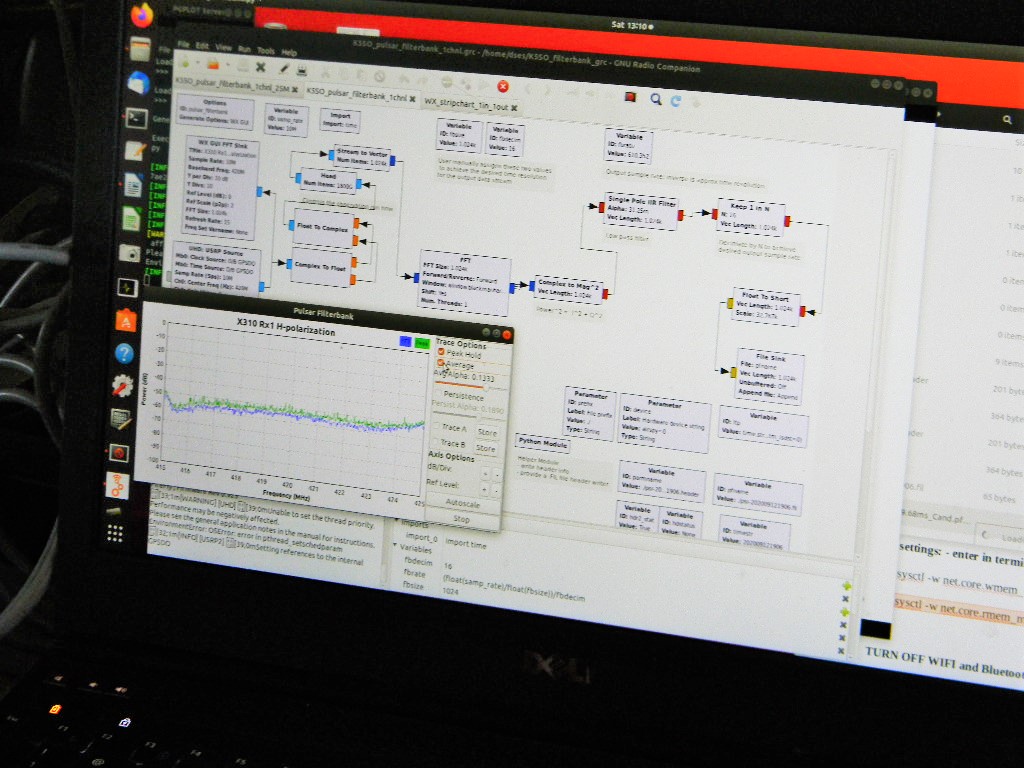
Because it makes the display much more user friendly, the display shows the visible stars and constellations as well. (You can click the image to enlarge it.)This screen is how we set our data parameters. And the display at lower left shows the signal coming in. The blue line is the data signal, across the bandwidth of 10 MHz, here centered at 420 MHz.
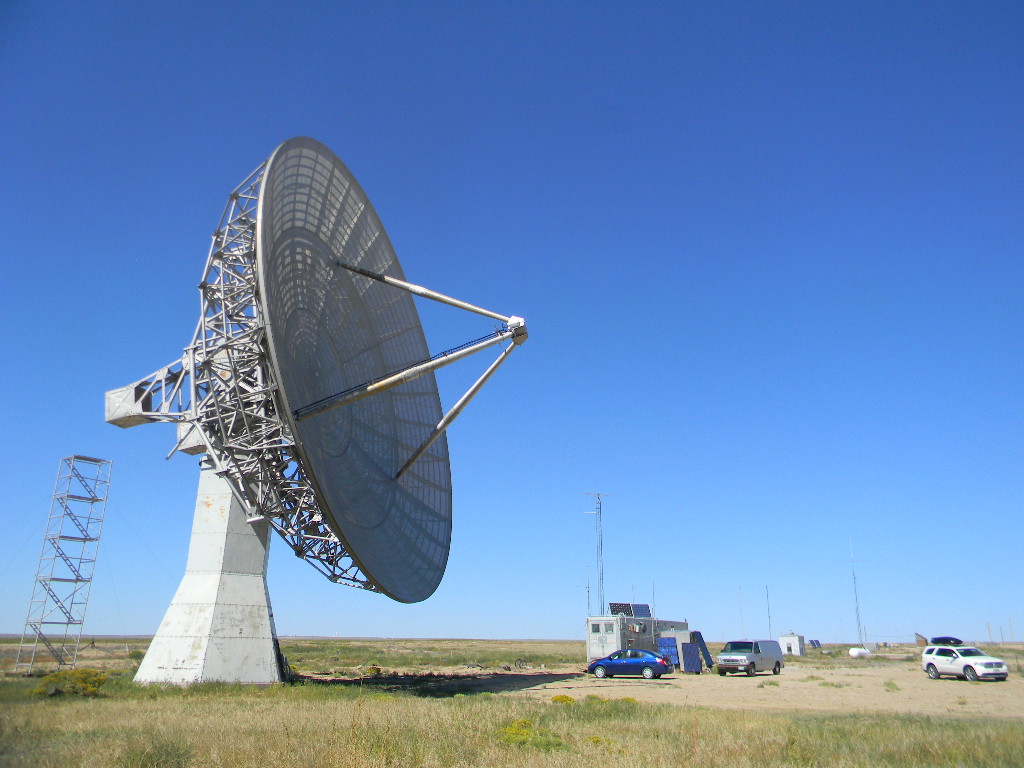
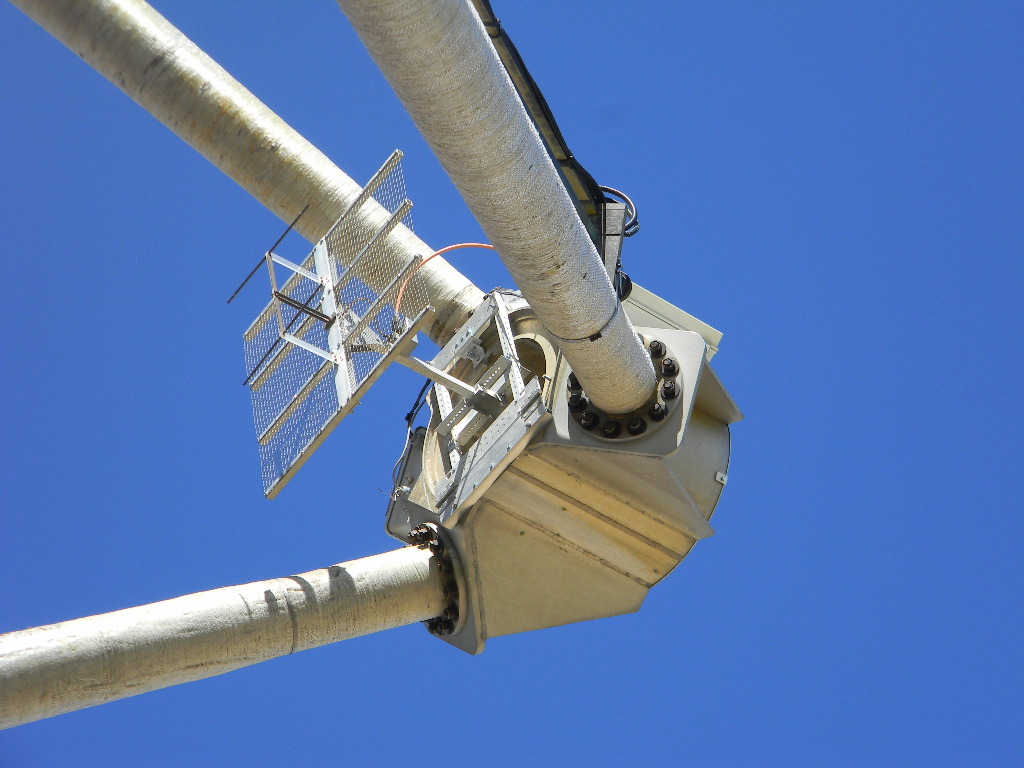
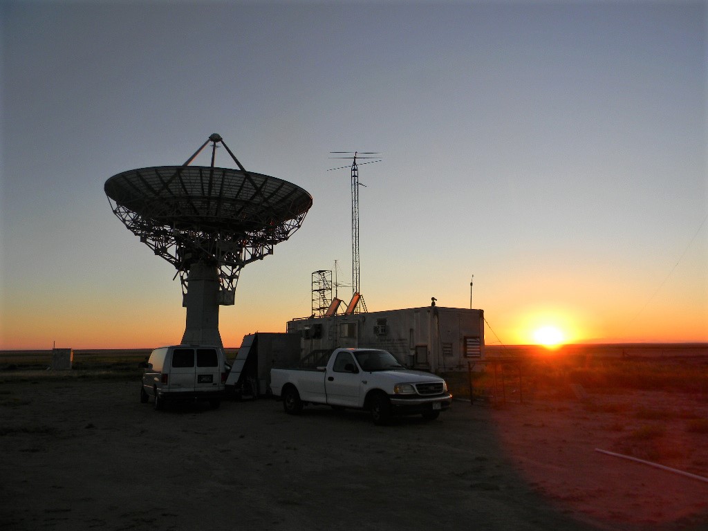
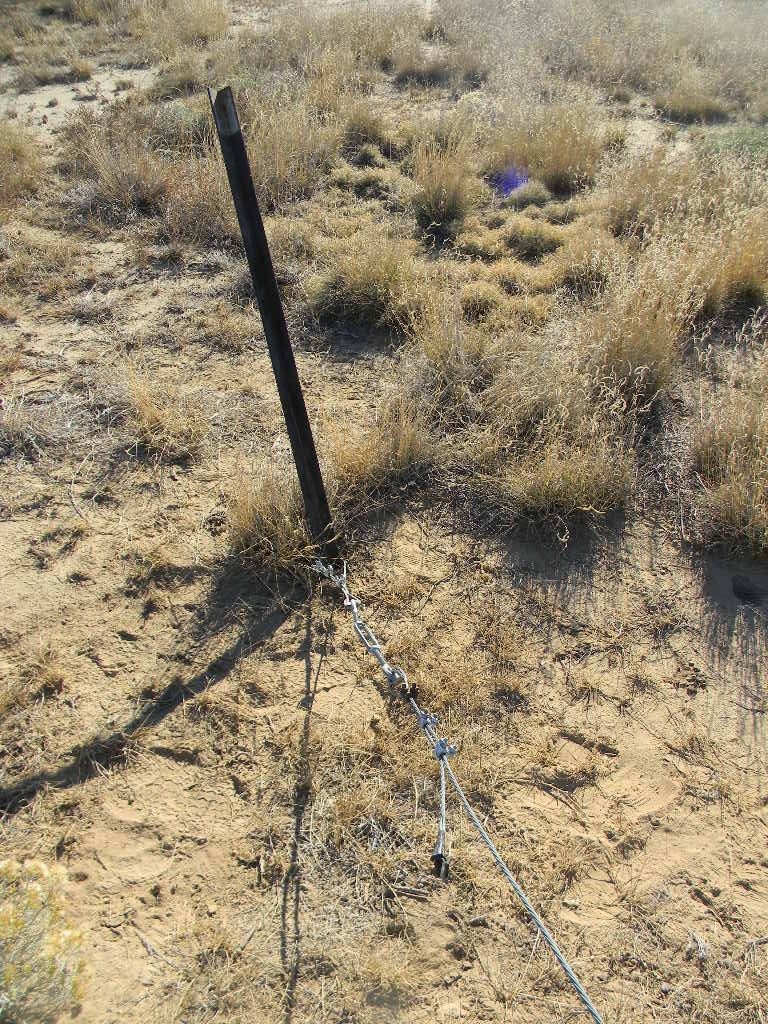
The green line shows the peak maximum of the signal over the course of the run. Earlier in the day we were seeing persistent radio signals, for us interference, at around 390, 406, 408, 410, and 432 MHz. We were concerned that one possible cause of problems with some of our data was the sun being close in angle to our pointing. We were never closer than 25 degrees from the sun. But we are wondering if the sun still might heat our preamplifiers at the feed focus of the antenna.The next set of photos are close-ups of the damage seen on the ham radio HF antennas. This is the tower with the 3-band Yagi. There is a slight tilt along the main boom.7 radials at the multi-band vertical antenna were also damaged. 5 severed at the lugs, which suggests metal fatigue from repeated moving in the wind. 2 were severed in their middles, which suggests some debris may have impacted those from the winds.Some of the fence damage by the bunker.The bunker ramp filled with tumbleweed again.Closeup of the 408 MHz feed and the feed mount at the focus of the 60 foot dish antenna. A closeup of the display we now use for pointing the dish antenna for astronomical observing. At the upper right, we can acquire the celestial coordinates from our database, or we can manually type in the needed data. The lower part of that window shows the actions the control system is executing, that is if it is slewing to an object, tracking, holding steady, or something else. The lower display shows the celestial sky, the coordinates, our antenna beam, as well as naked eye objects and constellations.The grain elevator in Haswell in the distance.
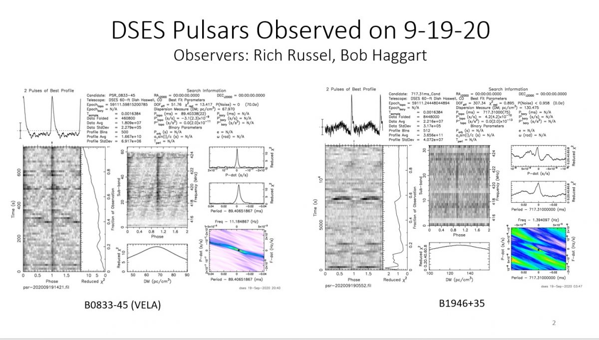
Bob Haggart and Rich Russel did an observation all nighter on Friday/Saturday (September 19, 2020, GMT) and observed 2 pulsars. VELA (B0833-45) is one of the strongest pulsars at 5 JY while B1946+35 is at 0.145 JY. DSES is one of the most northern amateur stations to detect VELA. We detected it in 15 minutes at 5 to 6 degrees elevation. This make 13 pulsars and puts us 5th on the international amateur pulsar hunter list. http://www.neutronstar.joataman.net/
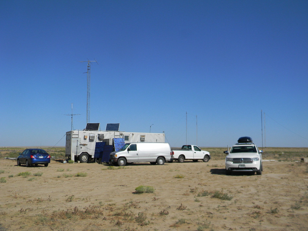
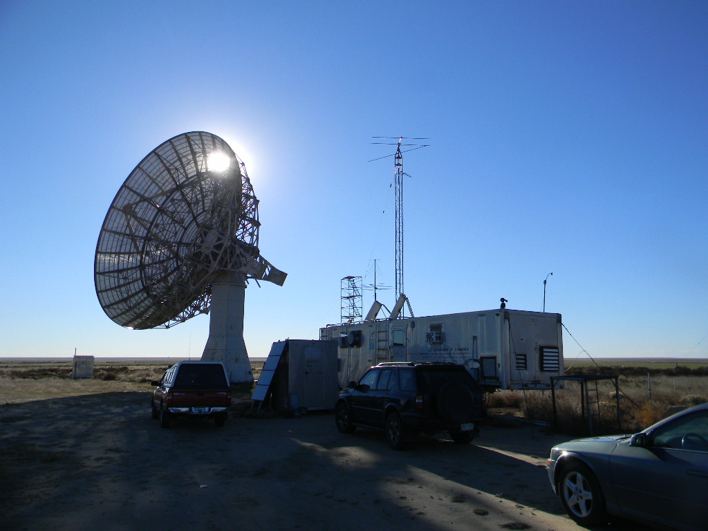
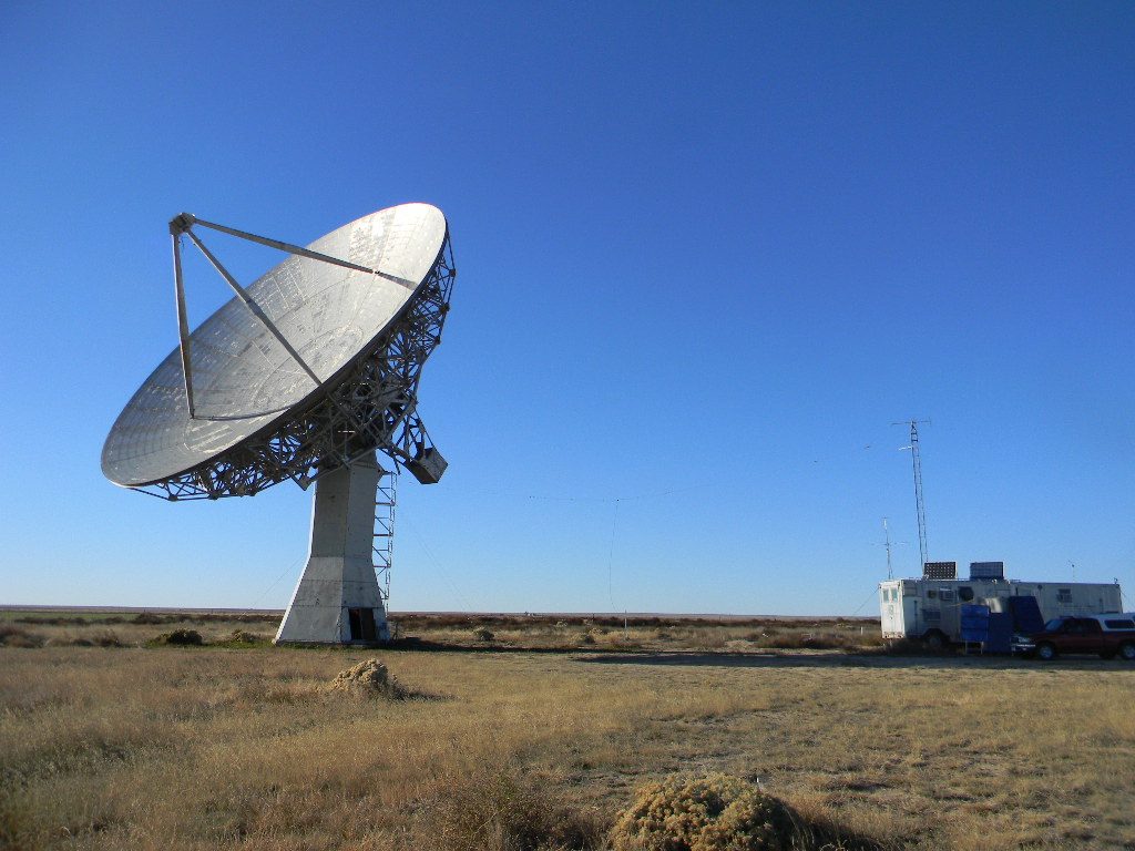
The DSES team of Rich Russel, Ray Uberecken, and Glenn Davis observed for pulsars on Saturday September 5, 2020 at the DSES 60-foot dish antenna at Haswell, CO.
The team successfully observed 5 pulsars which we hadn’t been able to detect before.
The success is attributed to the calibration of the antenna pointing system and the new automatic tracking system developed by the System 1 team.
We started with calibrating the azimuth of the antenna (it was 2.5 degrees off!) Elevation was good. Glenn put the offset in the auto tracking system and we were able to detect the B0329+54 pulsar within 30 minutes. (We use the B0329+54 pulsar, the first one we successfully saw last May, as a starting reference. If we can observe this, we know our system is working.) Every pulsar we looked at after that was detected – we just ran out of time for more!
It is possible we missed observing previous pulsars because our pointing accuracy was off.
We are pretty sure we observed the Crab pulsar. The last slide shows an analysis of the time between pulses we measured for the Crab pulsar, compared to the standard reference database.
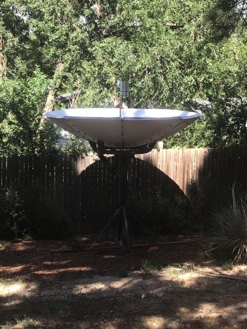
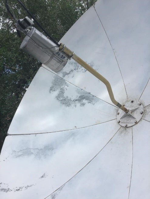
The DSES 9-foot dish is operational at Dr. Russel’s house in Colorado Springs. It is outfitted with a 1420 MHz feed with 2 low-noise amplifiers with over 40 dBi of gain and a noise figure of 0.35. The receiving system is a Spectracyber 1.
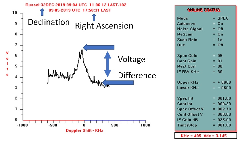
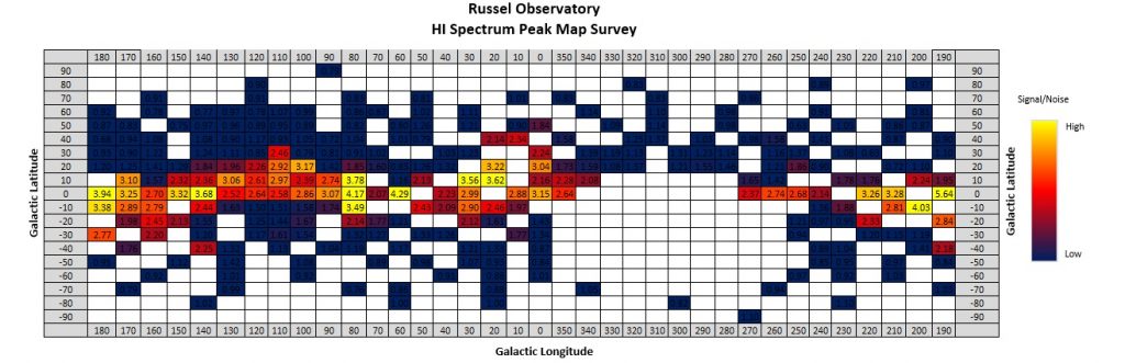
The output of the Spectracyber shows the relative peaks of hydrogen with a corresponding Doppler measurement.
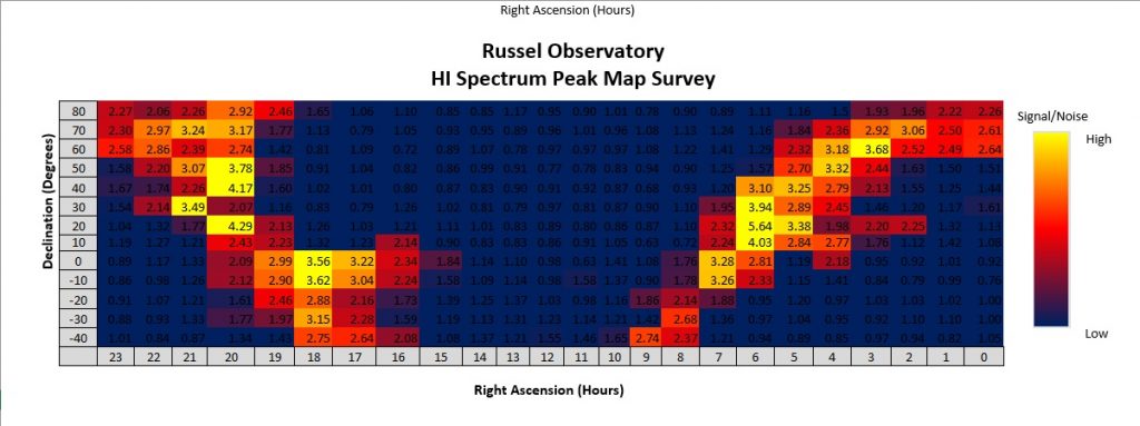
Dr. Russel performed a drift scan of the visible sky and plotted the relative peak hydrogen signals.
The hydrogen maps very well
to the visible Milky Way. The plot below converts the Celestial Coordinates
into Galactic Coordinates. Note that the peak hydrogen is concentrated near the
0 Galactic Latitude.
Special
Thanks to Ray Uberecken and Steve Plock for helping to set up the system.
These are the presentations from our DSES Science Meeting on November 26, 2018.
Dr. Richard Russel reported on the latest results from the Milky Way galactic rotation rate observations of November 16. Also, he compiled all of the observations of individual radio sources done with the 60-foot antenna with the Spectracyber 1420 MHz receiver. He includes descriptions of the objects and photos, as well frequency plot observations.
Prepared for the Deep Space Exploration Society by Skip Crilly. Revised November 8, 2018.
This is an updated revision of Skip Crilly’s slide set, originally presented last summer. Skip points out that the revision includes a summary of the pulses of November 2017 through November 2018.. Two newer NRAO 5690 plots in the presentation show the very stable performance of the telescope, and the narrower Plishner beamwidth.
This is a summary of our activities at the Plishner radio telescope site during the third week of October 2018. Steve Plock, Ed Corn, and Gary Agranat contributed to this report.
Participants this weekend were Gary Agranat, Paul Berge, Tony Bigbee, Ed Corn, Hans Gaensbauer, Dave Molter, Steve Plock, and Rich Russel.
Our plan for the rest of the year is to work at the site during the third weekend of each month. The Friday evening is devoted to astronomical observing, and the rest of the weekend is then devoted primarily to infrastructure and equipment work.
60-foot Antenna Observing, by Gary Agranat, WA2JQZ
On Friday afternoon and evening Rich, Gary, and Paul did 1420 MHz neutral hydrogen observing with the 60-foot antenna. The primary observing goal was to take regular measurements of the hydrogen signal along the Milky Way galactic plane at 10 degree intervals, from the galactic center to about 110 degrees (a little more than the first quadrant). The Doppler shift of the hydrogen was measured at each 10 degree point. From that, Rich later used some basic geometry to derive a velocity and distance from the galactic center for each measurement. A second goal was to observe several known, strong galactic radio sources that could be used in the future for calibration of our observations, and also to see if we are capable of observing those sources in a consistent way (without unknown biases). A third goal was to observe additional galactic sources as targets of opportunity, to see how well we do, and to also see what problems we hit.
Galactic plane observing started at about 5 pm local time, when the galactic center in Sagitarius had risen high enough in the sky for us to observe. The galactic plane and most of the other observing were done with the 60 foot antenna pointed along the meridian (180 degrees azimuth to the south and zero degrees to the north), in order to eliminate the Earth’s rotational motion in the Doppler shift measurements. We observed until about 10:30 pm, when the team was then quite tired. To warm us up during the evening, we made a batch of hot apple cider.
Details of the observations and results were discussed at the science meeting on Monday October 22nd, and those will be covered in a separate post.
– Gary WA2JQZ
60 foot dish antenna on Friday late afternoon, as the galactic plane observations started.
We’ll continue with the discussion of the weekend infrastructure work.
Saturday Infrastructure Work by Ed Corn, KC0TBE
Our first order of business was to re-service the toilet and spare in the outhouse. They now both have RV antifreeze for winter. Next installed was a portable heater for winter operations and I labeled all the breakers in the out house. I then labeled the doors with instructions for emergency exit and the safety pin for privacy at the main door.
With the help of Gary, Hans, and Paul we have the first 3 tower sections in place at the bunker, along with the first set of guy wires. [More about the tower below.]
-73’s Ed KC0TBE
DSES Site Work Report by Steve Plock KL7IZW, DSES President
Paul Berge worked on Friday, Saturday and Sunday. Because he travels from Lyons, Co. he prefers to maximize his efforts each visit. Also the weather window for the year is closing. I attempt to support his efforts as best as I can. Paul provided support for Rich Russel’s data acquisition which included galactic Doppler measurements. The team knocked off before midnight. Results have already been detailed in the Science meeting on 22nd of October.
On Saturday Ed installed a heater in the outhouse, winterized the RV toilets, and labeled the outhouse breakers.
During Saturday afternoon Hans, Ed, Paul, Steve and Gary all worked together to erect the new communications tower. The first set of guys were finished at 23 ft. by Ed Corn doing all the climbing. The majority of the rest of Saturday myself and Paul spent evaluating the elevation limit switch operation, including testing complete functionality with fault clearing via the built in override capability.
Later that day, Tony Bigbee showed up, and Paul and Steve supported subsequent hydrogen observations using the RASDR4 receiver.
The majority of Sunday was consumed by lubrication of the dish and adjustment of the azimuth drive chain. I also installed the conduit in the elevation bulkhead so that Bill Miller can complete his synchro wiring project.
Sunday Dave Molter worked into the night using the 500W floodlights and mixed over 1000lbs of concrete to try to prevent continued erosion in the ramp area. A big thanks to all who participated in this cooperative effort.
– Submitted by: Steve Plock, President DSES
Photos by Gary, from Friday and Saturday:
Position of the 60-foot antenna as it is pointed due south, at 180 degrees azimuth along the meridian.
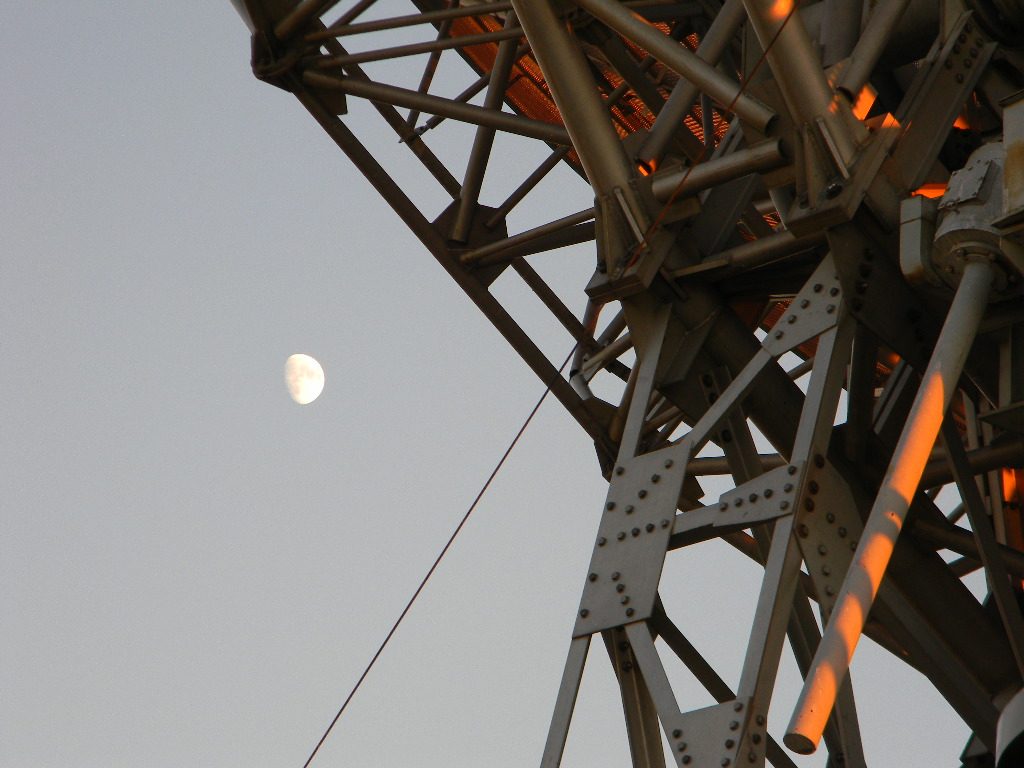
The Moon with the 60-foot antenna.
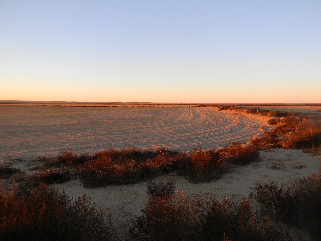
View from the base of the dish antenna, looking towards Haswell.
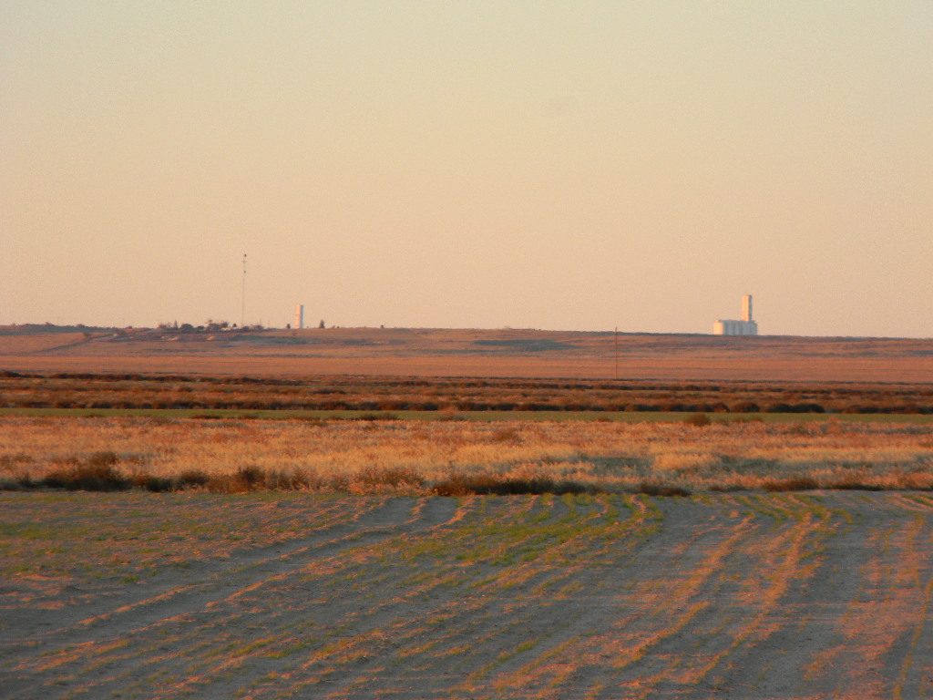
Haswell as the sun set Friday evening.
Pikes Peak and Cheyenne Mountain were visible on the horizon, about a hundred miles to the west-northwest.
Work Saturday morning at the outhouse.
Work at the outhouse, including labeling.
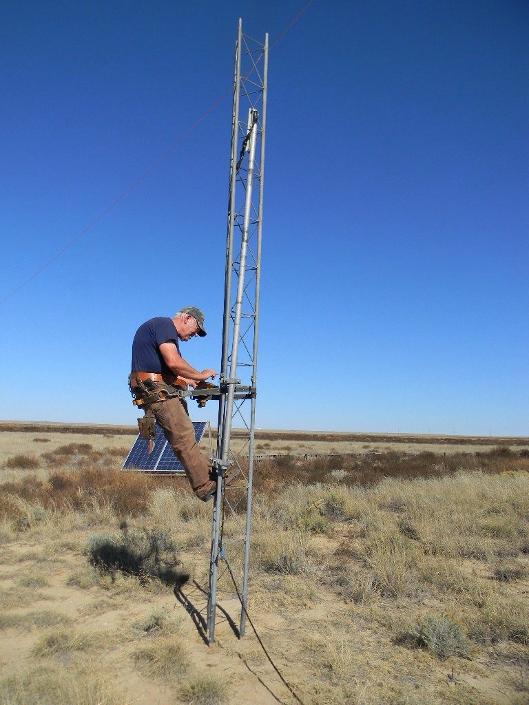
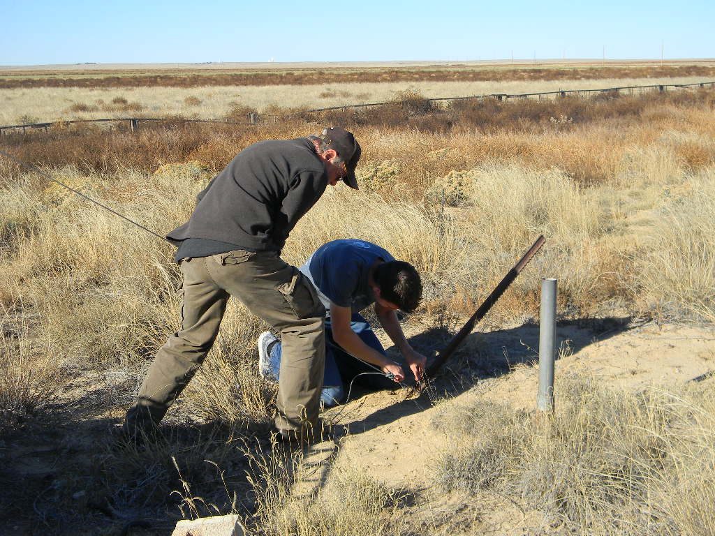
Hans helping Ed unload tower sections and a jin-pole, for building up the ham radio communications tower at the bunker.
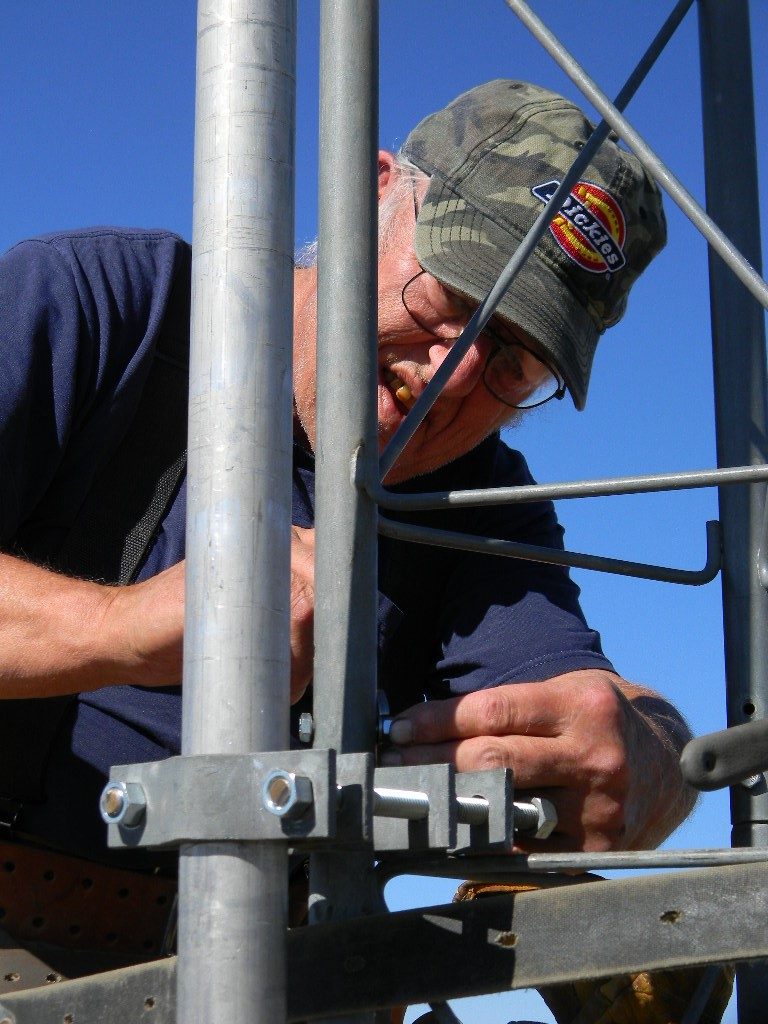
The first section of the tower had already been installed during the last work trip. Here Ed is safely secured to the tower after the second section has been hoisted with the jin-pole, which is also temporarily securely attached to the tower. He is fastening the bolts of the second section on to the top ends of the first section. He did this again with the third section.
Ed fastening the bolts of the second tower section on to the top of the first.
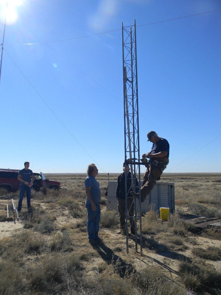
The team standing ready as Ed works on the tower. Hans is standing by the third tower section.
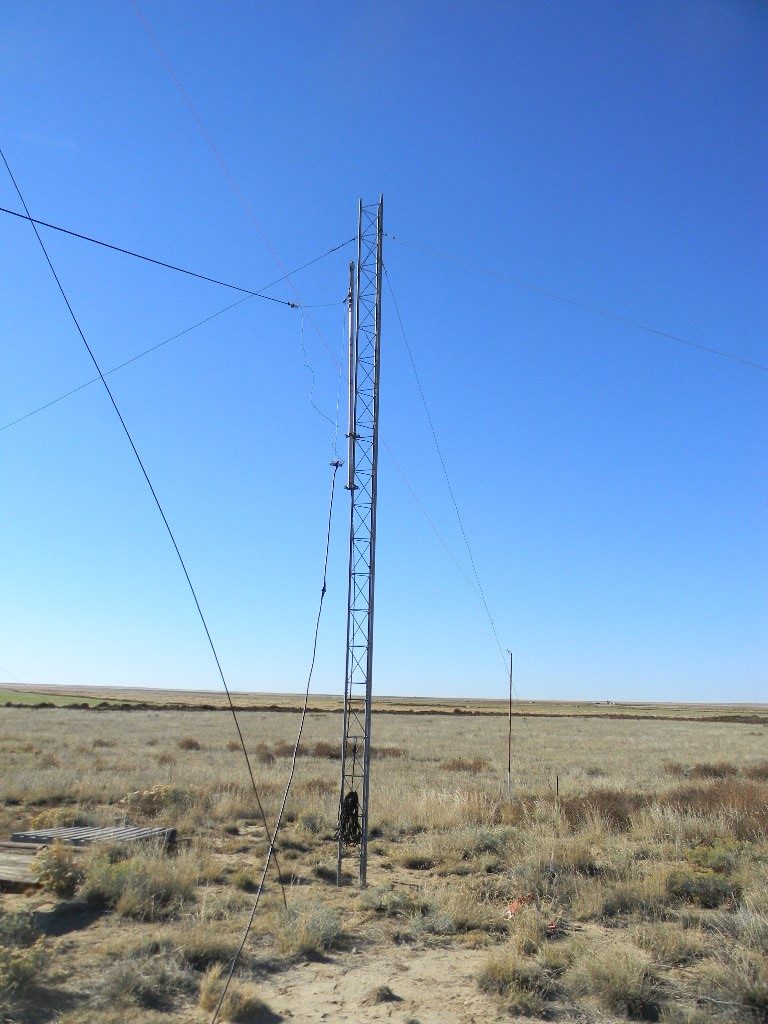
The tower at left with the third section up. A 6-meter delta loop antenna was hung from the tower to the doghouse. Stainless steel guy wires were also extended from the third section, per tower specifications.
Hans, Paul, and Gary installed supports for the guy cables, at one-third intervals around the tower.
Hans and Paul securing one of the guy wires at the ground support.
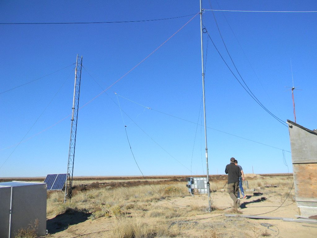
Configuration of the tower with 3 sections, until work resumes next time. The current plan is to install one more section with a rotator. The rotator shaft will have at least a triband HF yagi antenna and a 6 meter directional antenna for meteor scatter. Also, small horizonal supports will be added to support the 80 and 160 meter dipoles, currently supported at that position with a pole.
These are the slides from Dr. Richard Russel’s presentation about the radio astronomy observations conducted at the Plishner site during the previous Saturday, September 22. The observing period was chosen for Saturday afternoon, when the Milky Way around the galactic center was starting to rise high enough in the east. Observations were done using the Spectracyber at the 1420 MHZ neutral hydrogen I (HI) frequency.
Goals for the observing included 1) using our in-house Radio Astronomy Guide as an observing reference, 2) seeking strong enough sources listed in our guide that could serve as calibration references, 3) scanning perpendicularly across the plane of the Milky Way to observe changes in hydrogen signal while pointed inside and outside the galactic plane, 4) starting a series of doppler shift measurements along the plane of the Milky Way at galactic longitudes 10 degrees apart.
Some sources were found, but some were not. Among those found were Centarus A, Sagitarius A, and Virgo A. A number of peaks in the hydrogen signal were seen where we didn’t have any reference information that sources were present. The scan perpendicularly across the galactic plane showed the higher concentration of hydrogen in the galactic plane. We likely also detected the weaker signal of hydrogen known to be above and below the plane in certain regions. For this observing set, some sources like Sag-A were so strong that they oversaturated the voltage scale we had initially set. Doppler shifts were measured at 5 points, 10 degrees apart, along the galactic plane. Please see the slides for details.
Please click the link to see the power point slide show.
Participants: Steve Plock, Ed Corn, Rich Russel, Dave Molter, Gary Agranat.
Summary and photos by Gary Agranat.
We worked at the Plishner Radio Telescope site on Saturday August 25, 2018. One motivation was to proceed with needed infrastructure work before the cold of winter returns. Another motivation was to follow up on the observations we made during the Open House with the 60-foot antenna. In addition, the antenna tuner for the bunker ham radio station was still not running, and needed to be checked. Here is a summary of what we did, with some photos.
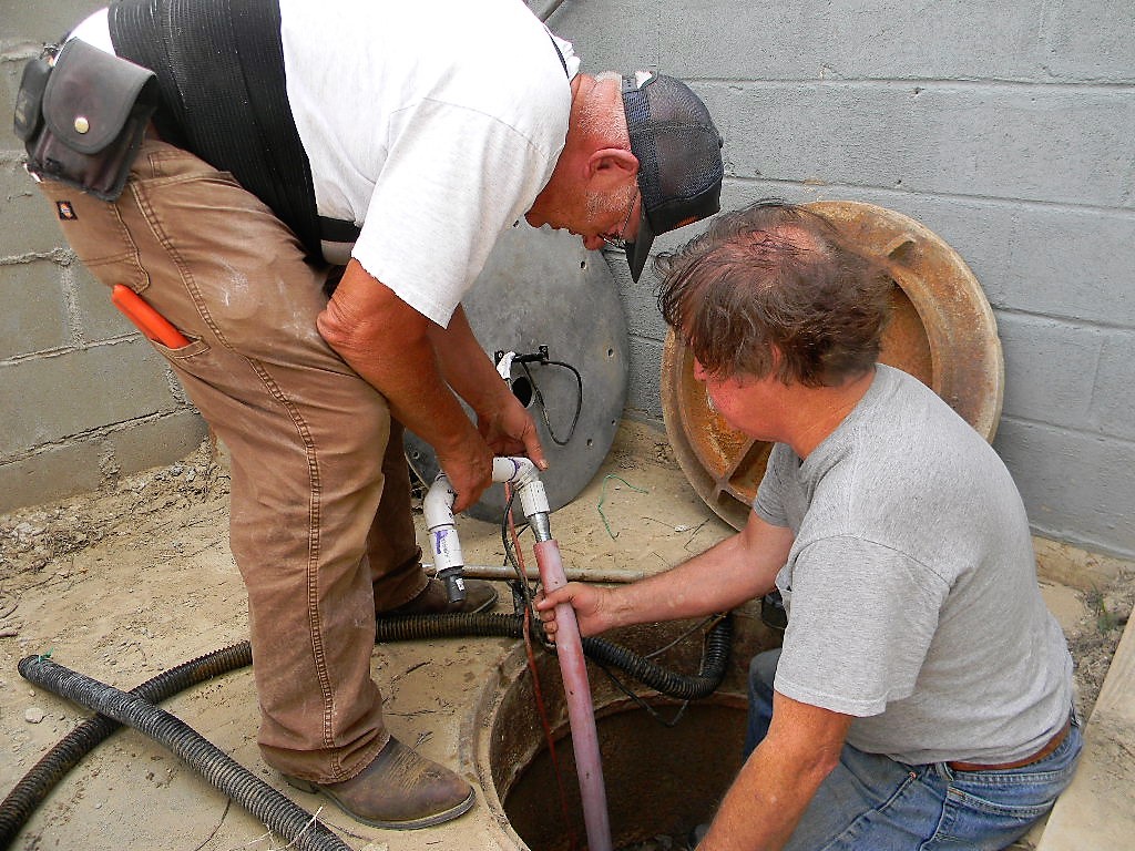
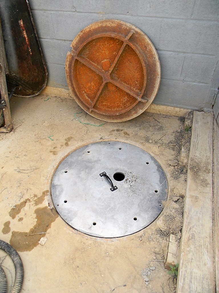
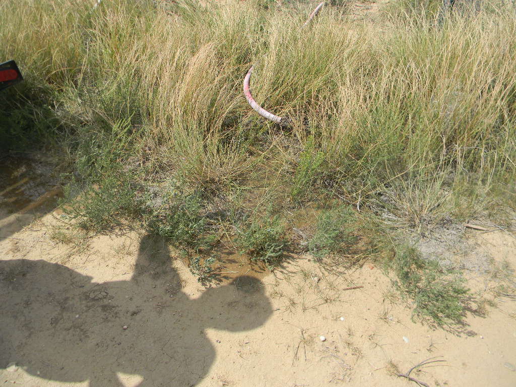
1. Ed and Steve replaced the outflow hose from the ramp sump with one more durable (including durable against mice). Ed tested that the outflow did drain away from the ramp area. We placed a new aluminum manhole cover on the sump access (vs the original steel one), fabricated by Steve.
2. Ed moved the Internet hotspot to the bunker. The hotspot was used by Gary while testing and operating the ham radio station.
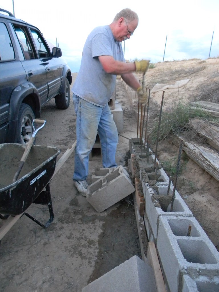
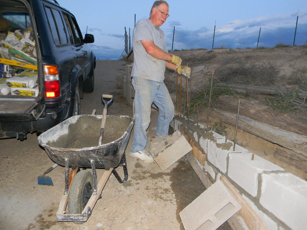
3. Dave brought 20 x 60-pound bags of cement, and used all of them to continue to repair/rebuild the ramp retaining wall. He made considerable progress extending the base of the wall. The higher the base of the wall reaches up the ramp, the less rain sediment will clog the sump pump. Dave stayed until late in the evening, until around sunset. Gary stayed with him and gave some help.
4. Rich brought the SpectraCyber 1420 MHz Hydrogen Line Spectrometer, and used it to continue to test the functioning and ability of the SpectraCyber together with the System 1 pointing system on the 60-foot antenna. Rich later showed Gary how to steer the dish antenna, and how to measure and record neutral hydrogen data. By the end of the day we located and measured several radio sources in the Sagitarius region. And we made a systematic scan almost perpendicular to the Milky Way galactic plane, in order to measure neutral hydrogen while pointing away from and in the plane. A more detailed discussion follows later in this post.
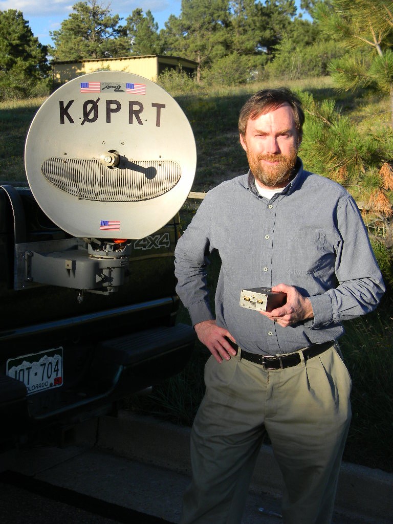
5. Gary tested the setup of the newly installed auto tuner for the FT-897 in the bunker ham station. With some adjusting and checking of cable connections, the tuner was found to be functioning OK. Gary took the opportunity to operate K0PRT in the QSO Parties this weekend for Kansas, Ohio, Hawaii, and for the US & Canadian islands, making about 30 contacts, on SSB and CW, on 40, 20, and 15 meters. Signal reports were mostly good, which seemed to indicate the combined FT-897 + tuner system is working OK. Gary wrote some Guidance Notes for using the tuner, and left those next to the tuner.
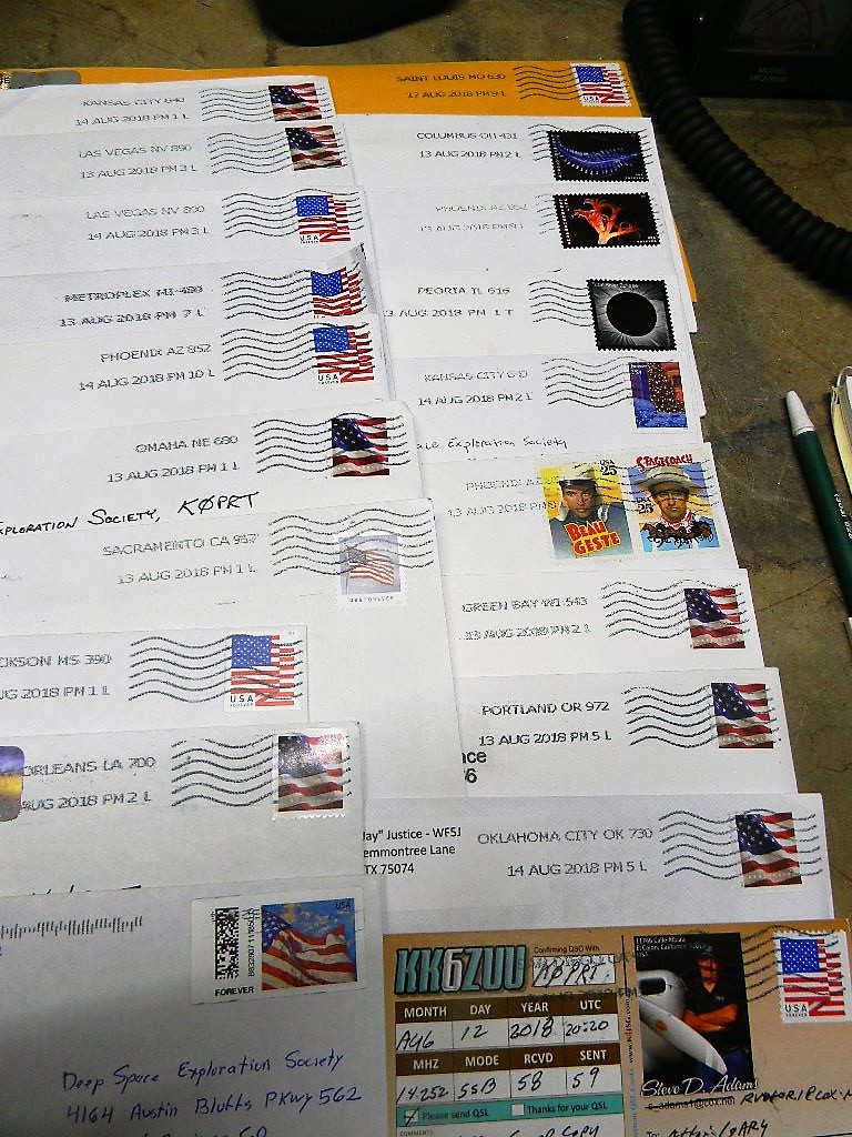
6. We received 20 QSL cards in the mail from the Open House special event station. Myron passed them on through Ed to Gary. Gary responded to all of them, and sent in the mail our QSL card responses to all by Monday.
Next are some photos of our work. Then follows a more detailed discussion about the SpectraCyber observations with the 60-foot antenna.
Ed and Steve replaced the outflow hose from the outer sump pump. The new hose has a more robust thick wall to protect it.
Steve fabricated a new manhole cover for the outer sump. It is made of aluminum, and is much easier to handle than the original steel cover (seen leaning against the wall). The holes allow water runoff to flow into the sump during rains.
The exit of the sump outflow hose reaches well away from the ramp area.
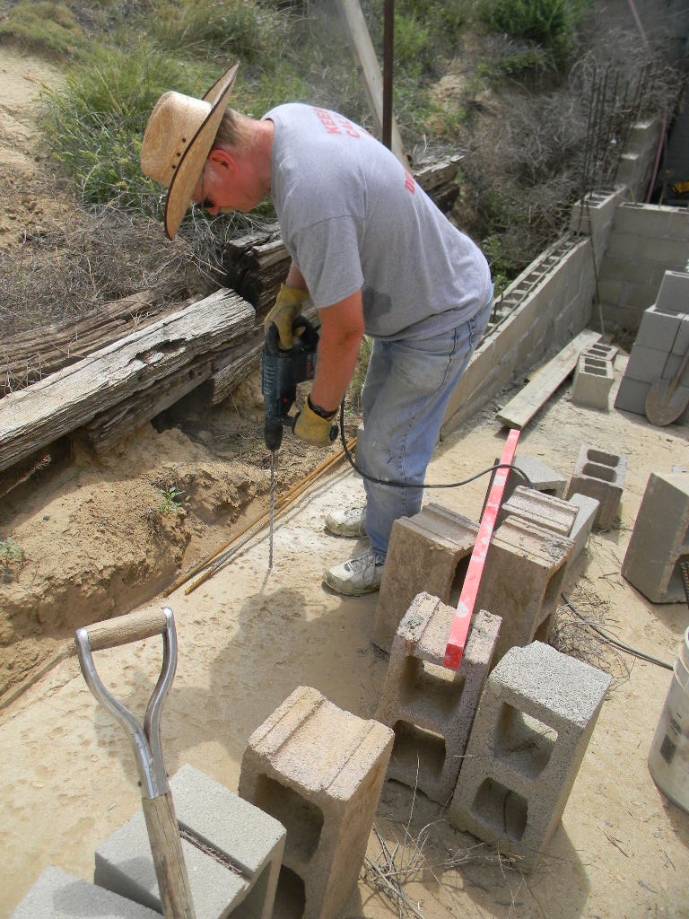
Dave Molter devoted the afternoon and evening to continuing the repair of the ramp wall. Here he is drilling holes for the steel reinforcement bars.
Cutting the re-bars to suitable sizes.
Mixing the cement. Dave brought 20 x 60-pound bags of cement and cement blocks to continue the wall repair.
View of the wall repair work, late into the afternoon.
View of the wall repair work, late into the afternoon.
View of the wall repair work, late into the afternoon. You can see by how much more the wall has been extended. One purpose of the wall is to control the erosion of the soil on the side, and prevent rain runoff with sediment clogging the sump pump at the base of the ramp.
Some rain showers passed just to the south late in the afternoon, as was in the NWS forecast.
Dave stirred the cement inside the blocks, to eliminate the air pockets.
Dave worked on the wall until sunset, and used all of the 60-pound cement bags he had brought. It was a lot of physical work.
SpectraCyber observations with the 60-foot antenna
Rich brought the SpectraCyber 1420 MHz Hydrogen Line Spectrometer, to follow up on the successful observations we started to make with the 60-foot antenna during our Open House 2 weeks before. We used the System 1 pointing system. I later joined him by mid afternoon, after I finished my other work, and this is a report of what we did.
We started by searching for several sources with flux density values higher than 200 Janskies. However, at first no sources were found. The plane of the Milky Way was at that time very low along the southern horizon. There were few strong sources on our list available to look for at that time.
A little later, we just about ran into the Milky Way without looking for it, when the galactic plane rose higher. The signal trace of the SpectraCyber indicated the change: pointed away from the galactic plane, the signal trace stayed near about 3 volts, varying probably with noise, but not by more than a volt. Once pointing at the galactic plane, the voltage trace increased from about 5 to 7 volts (up to about 4 volts above the noise floor). The signal consistently showed a peak at about the center of the trace, at about the frequency of neutral hydrogen. We have not calibrated the SpectraCyber, and so we don’t exactly what frequency we were peaking. (The actual spectral line frequency is 1420.40575 MHz. And we may be seeing some doppler shift in our measurement.)
We then looked for several strong sources in the Sagitarius region, which by then had risen. We successfully found several, including:
Sagitarius A, the center of our Milky Way galaxy. The radio emission is thought to be from the secondary effects of a black hole there.
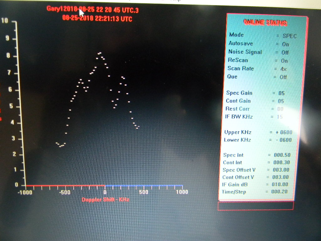
CTB 37, a supernova remnant about 20,000 light years away (see https://www.nasa.gov/mission_pages/chandra/ctb-37a.html.) Our signal trace showed three peaks through most of our scans. Our interpretation is that the central peak is the original supernova remnant. The other peaks would be the doppler-shifted material outflowing away and towards us, following the supernova explosion.
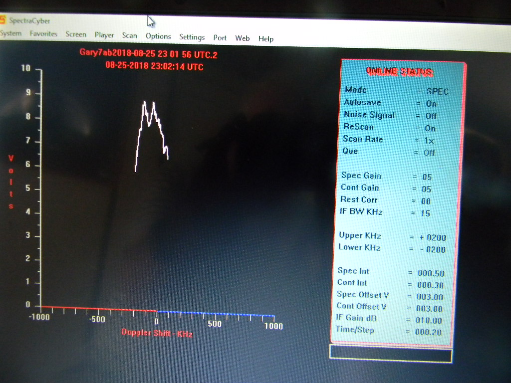
The Sagitarius Star Cloud Messier 24, with a colder hydrogen cloud closer along the line of sight that absorbs some of the M24 hydrogen signal. This is the radio source Tony Bigbee pointed to during our Open House 2 weeks earlier. The signal trace has a distinctive dip, which had been identified in data from the Parkes Observatory in Australia. And as Tony has discussed, was used in the past by the RASDR2 team as an engineering detection test. The dip in signal is interpreted as a hydrogen cloud along the line of sight that is colder than the background source. It absorbs the background signal and then reradiates it out, but in all directions, hence the net signal to us is reduced. We used the RA & Dec location coordinates recorded during the Open House. We found the source again without difficulty.
We used the System 1 computer display to read the angles our 60-foot antenna was pointed to. The display showed coordinates in both azimuth & elevation (Earth ground reference), and Right Ascension & Declination (celestial sky coordinate reference). We turned the antenna with the manual steering controls. At this time we do not have automatic tracking ability. But we were able to reasonably stay on our targets with continual manual adjustments. What we more often did was we found our source, then allowed the antenna to scan at the set elevation as the Earth rotated, and as a result get a short scan along a line of Declination. We then moved the elevation up and down slightly, to see differences in the scans a little north and south. We used this technique also to hone in on targets.
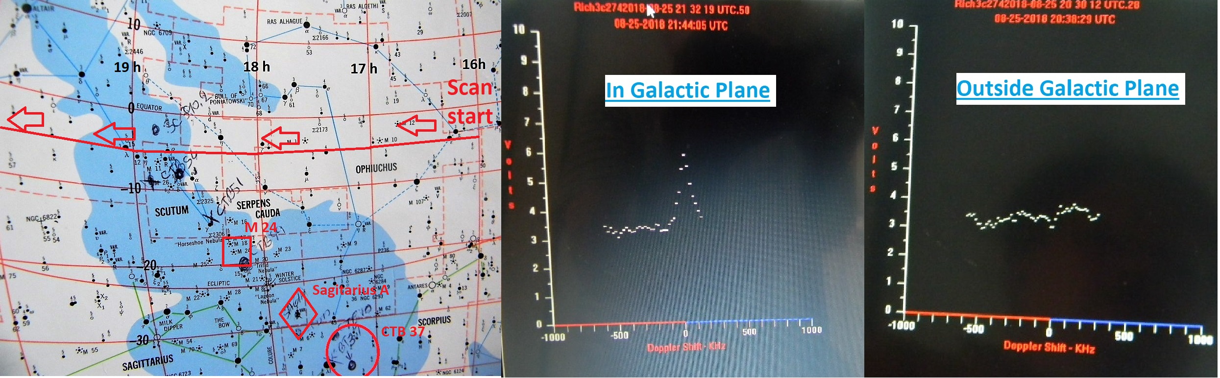
We then manually scanned across the Milky Way galactic plane, to obtain a slice from 16 to 20 hours Right Ascension, along the declination of -05 degrees. We stopped at intervals of 30 minutes Right Ascension (e.g., 17h 00 min, 17h 30 min, 18h 00 min, …), to let the SpectraCyber take full scans.
Our scan cut a steep acute angle through the width of the galactic plane, going across the constellations of Ophiuchus, the north edge of Scutum, and the southern part of Aquila. We therefore started and ended at angles pointed “above” and “below” from the galactic plane, and scanned across the galactic plane in between.
Since we were pointing to the southeast (and not due south), if we moved azimuth while maintaining elevation, the declination still changed. And so to keep on the -05 degree declination line, we had to adjust azimuth and elevation together.
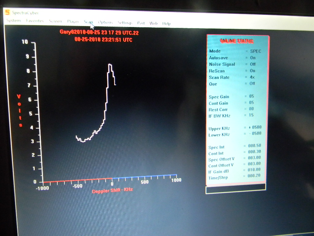
The SpectraCyber display showing the signal we saw at the location of Sagitarius A. The scan traces frequency from 500 KHz below to 500 KHz above the 1420 MHz neutral hydrogen frequency. The vertical axis measures the strength of the received signal, in volts. Sag-A is believed to be a super-massive back hole at the center of our galaxy. The radio source is thought to be created by the secondary effects of infalling matter at the surrounding accretion disk, and perhaps also from material ejected at the rotational poles.
Our scan at the location of CTB 37, a supernova remnant about 20,000 Light Years away in our galaxy. We think the original star that exploded as a supernova is the central peak. The two other peaks at offset doppler shifts would be the shells of gas flying towards and away from us, from the explosion.
The Sagitarius Star Cloud, also known as Messier 24, with a colder dark gas cloud closer along the line of sight, absorbing some of the hydrogen signal from M24. This is the object Tony Bigbee observed during our Open House. We were able to locate it again without much difficulty, using the coordinates we recorded then.
A composite image showing a chart of the part of the Milky Way we scanned across. Shown with it are example signal traces away from and in the galactic plane. The shaded blue areas on the chart are where the Milky Way is in visible light. I wrote in red the path of our scan. Also written in are the locations of Sag-A, CTB 37, and M 24. (Click for a full sized image.) Notice that our scan cut across an apparent gap in the visual Milky Way, around 18 Hours RA. But we saw an increase in neutral hydrogen already by 17 H 30 minutes (to the right, earlier in our scan). That indicates the apparent gap is just caused by intervening dust blocking the visible light of the stars. The radio measurement of neutral hydrogen over that area shows the galactic plane is in fact there.
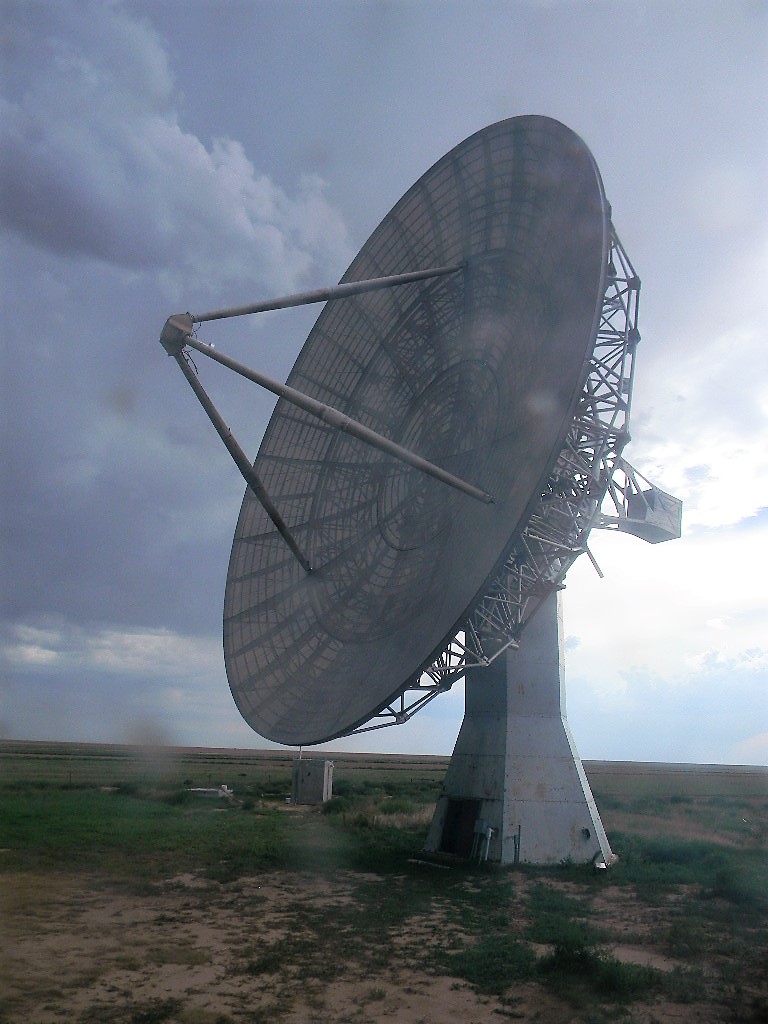
A view of the 60-foot antenna while we were scanning across the Milky Way. A rain shower was passing just to the south.
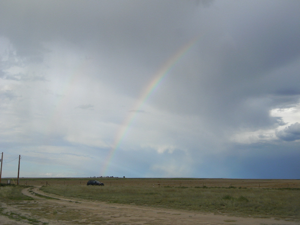
Rich Russel recording notes during our observations.
We saw a rainbow as Rich left.
QSL cards we received in the mail from our Open House special event station operation. : )
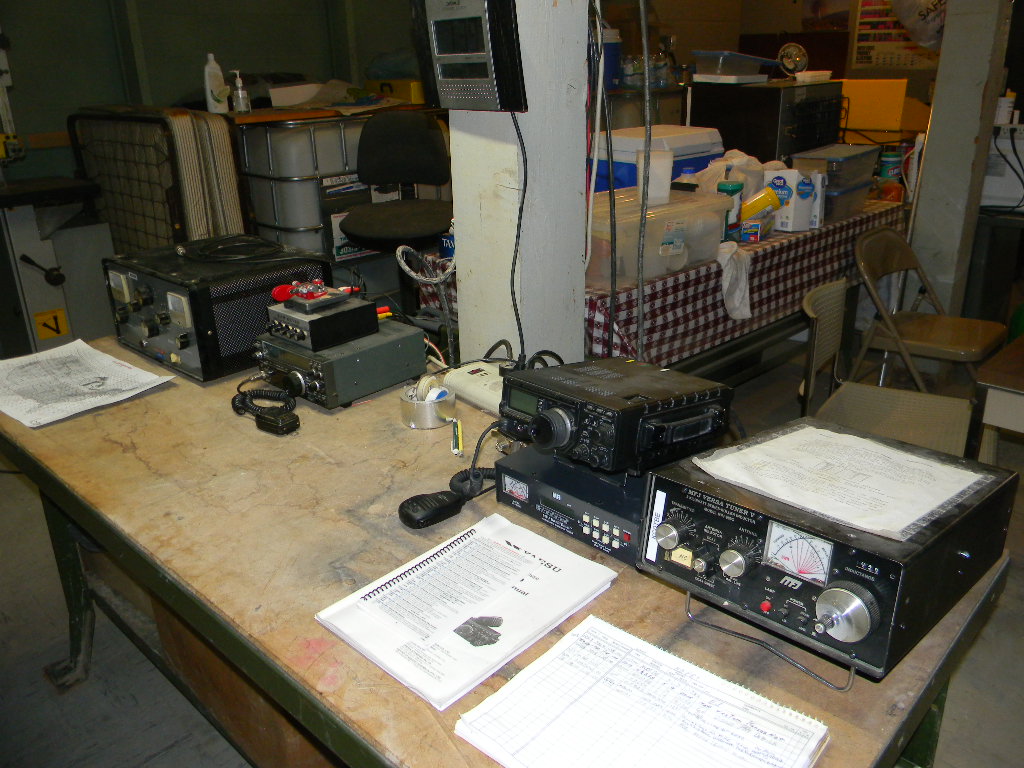
Our current ham radio station set-up in the bunker. The auto tuner is below the Yaesu transceiver and is functioning normally. For this location we have dipoles for 160 and 80 meters, and a multi-band trap vertical antenna for 10, 15, 20, 40, and a portion of 80 meters. The antennas are tuned well enough that we don’t require tuners for most of the spectrum on those bands.
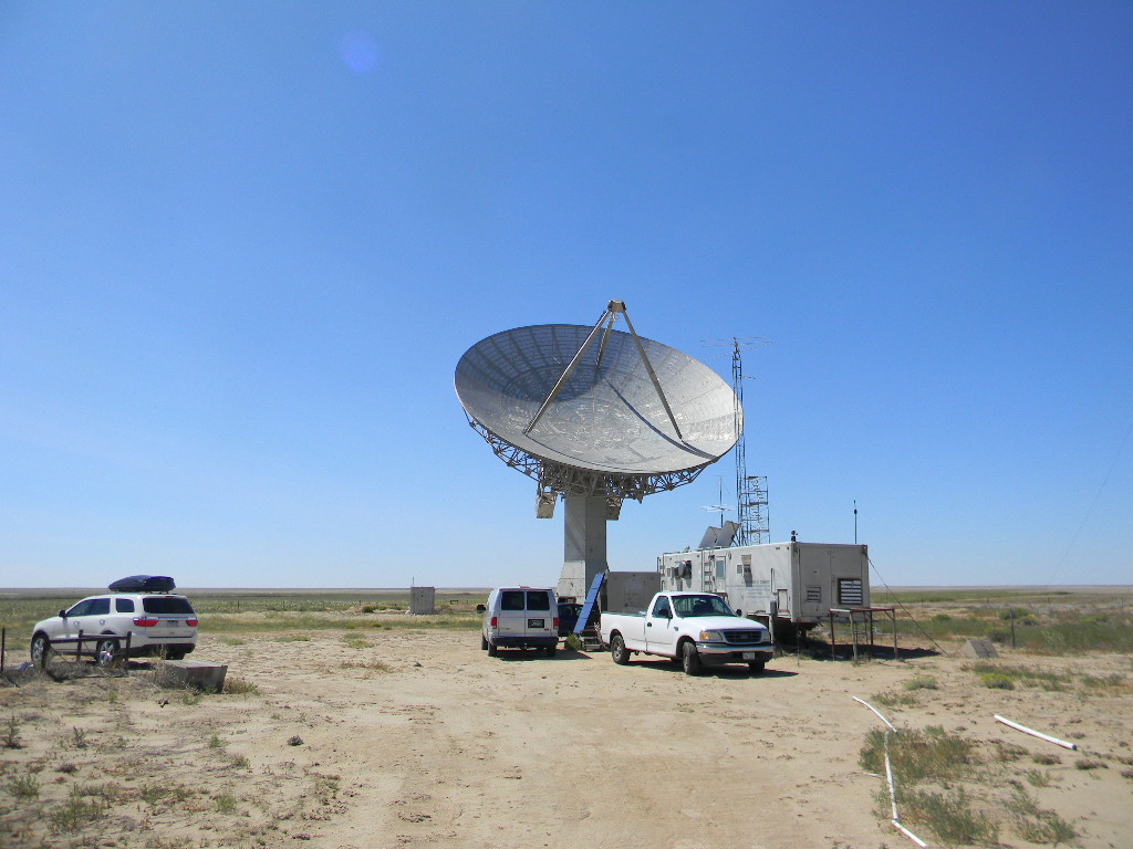
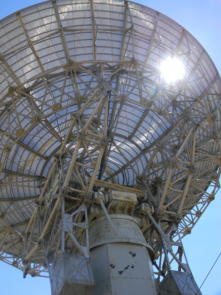
60-foot antenna, in stowed position.
DSES Science Meeting August 27, 2018 Follow Up
On the following Monday we had our monthly DSES Science Meeting at the home of Rich Russel.
At the meeting we discussed the observations we made with the 60-foot antenna two days earlier.
Tony Bigbee then also presented deeper details about his RASDR4 (Radio Astronomy Software Defined Radio). And he gave us more background about the earlier RASDR2 observations of Messier 24, with the dip in frequency. And he showed how he researched the earlier Parkes observatory data to find useable results and plots for us to compare to.
Tony Bigbee with his RASDR4 (Radio Astronomy Software Defined Radio), at the DSES Science Meeting August 27, with Steve Plock’s 10 GHz mobile antenna.