2020-10-26 DSES Science Meeting Notes: by Bill Miller
We had 14 participants in the virtual science meeting today: Thanks everyone for joining.
Participants: Dr. Rich Russel, Ray Uberecken, Chad Carter N0ZMG, Don Lewis, Matt Mathews, Bob Haggart, Michael Nameika, Gary Agranat, Jonathan Ayers,Floyd Glick, Don Latham, Myron Babcock, Ted Cline on Phone, Bill Miller
Also see the Zoom Video Recording for more detail:
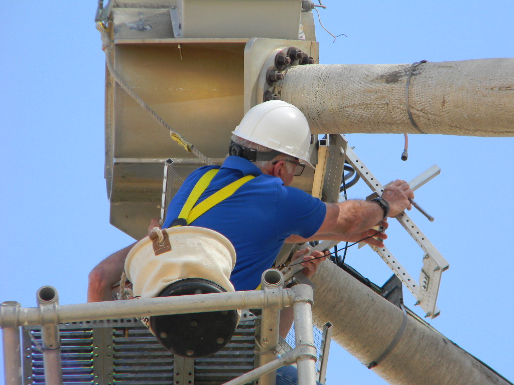
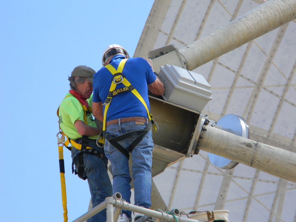
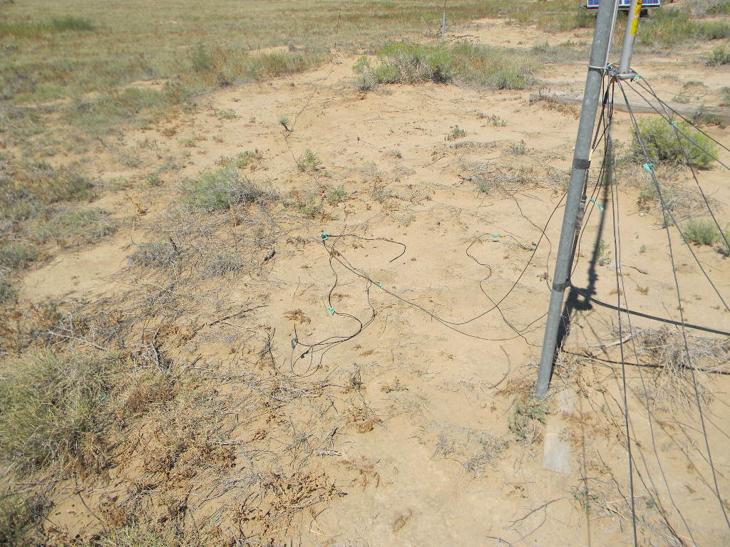
Problem with the 1296 MHz feed last weekend. Took down the Feed amplifier and found the unit was stuck in the transmit configuration due to a failed FET in the Relay driver. Fixed this and added a gate protection resistor to solve the problem.
A second issue was discovered with one of the coaxial swivel joints that failed on the feed lines. Will find a new swivel joint or alternate method of coupling the coax while allowing for the cable wrap.
See slide 4 of Rich’s slide presentation above.
Gary EME report.
See report of contacts in slide 5 of Rich’s Power point presentation above.
On November 28 and 29th there will be another EME contest under nearly a full moon.
Nov 27 – 28 Moon Rise 3:19 PM set at 5:03 AM
Nov 28 – Nov 29th Moon rise 3:47 PM to about 6:03 AM
We will benefit by organizing the operation trip, to utilize our time while the moon is overhead with multiple operators.
Morse code is simple and effective. Can be done with the computer keyboard or with a keyer.
Simple protocol of multiple repeats on Call sign, signal report and acknowledgement should be followed.
Signals experience polarization rotation, we therefore circularly polarize our signal.
Operation on JT65C will be added.
Operating EME is an experience you won’t forget
Astronomy at Hydrogen Line 1420.406 MHz: See Rich’s PPT presentation page 6 to end.
SARA “Radio Astronomy in a Box” costs about $250 and is a great platform for a science fair project. Rich has one for evaluation and will lend to a worthy student.
2.4 G dish
Stellarium planetarium software
Can be used for science fair
Don’t download the SW, as it has a virus.
Rich has another source of virus free SW.
We have a new student member, Michael Nameika who is a student at UCCS interested in Astrophysics and Radio Astronomy. He has been working with Professor Floyd Glick at the PPCC observatory and with Steve Plock. Welcome, Michael.
Myron Babcock, DSES Treasurer, has received a very generous donation of a Yaesu FT-736R from N6KN, Rocco Lardiere in California. He also triple boxed the unit and paid the FedEx postage to ensure that it arrived in great shape. This will make an excellent addition to our radio resources and backup to our high band EME and Tropo communication. Thank you, Rocco.
By Gary Agranat, with Myron Babcock and Glenn Davis. Videos by Bill Miller.
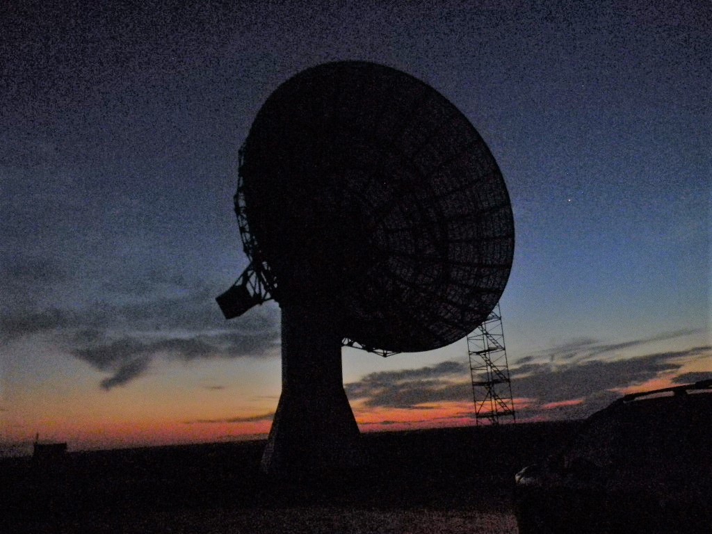
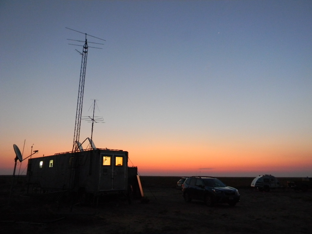
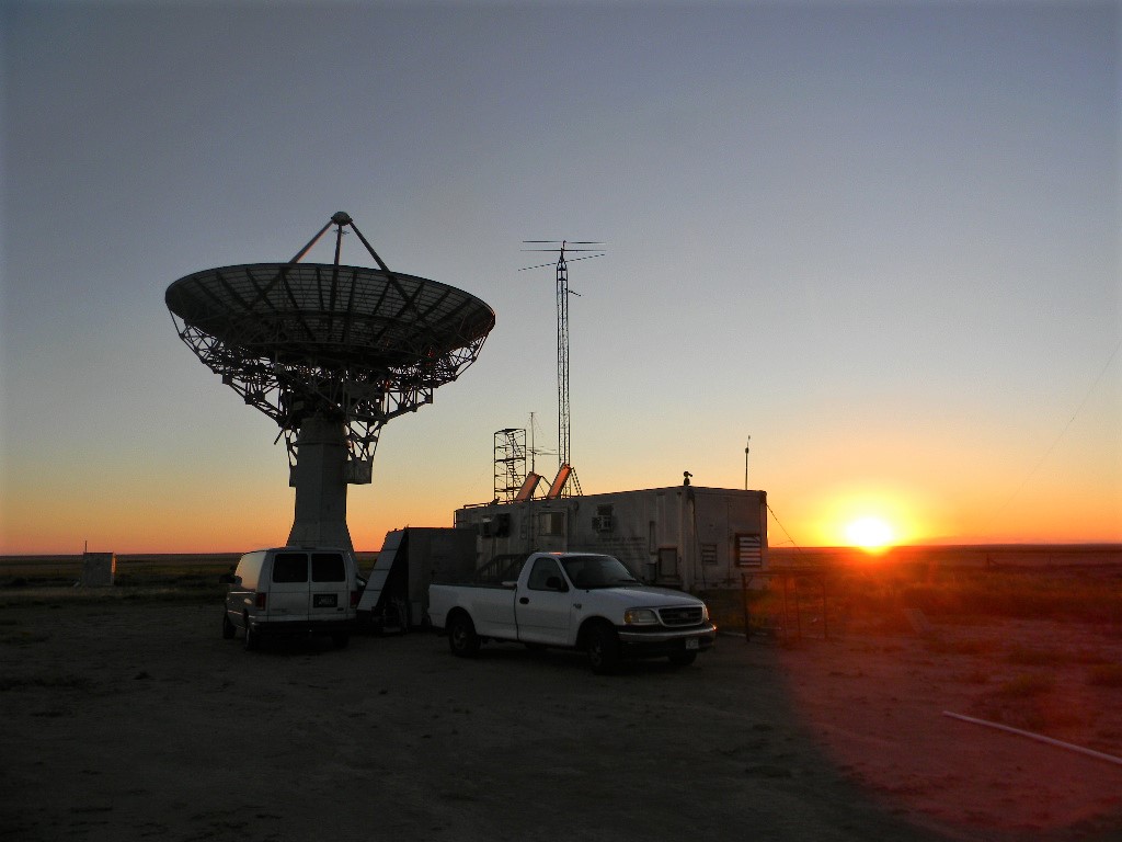
Friday evening at sunset as the team prepares for our first EME attempt overnight. Photo by Gary Agranat.
On Saturday October 10, 2020 we succeeded in making our first Earth-Moon-Earth (EME) Moon Bounce communications. We succeeded at our first attempt. This accomplishment was several years in the making, thanks to the work of many members, past and present.
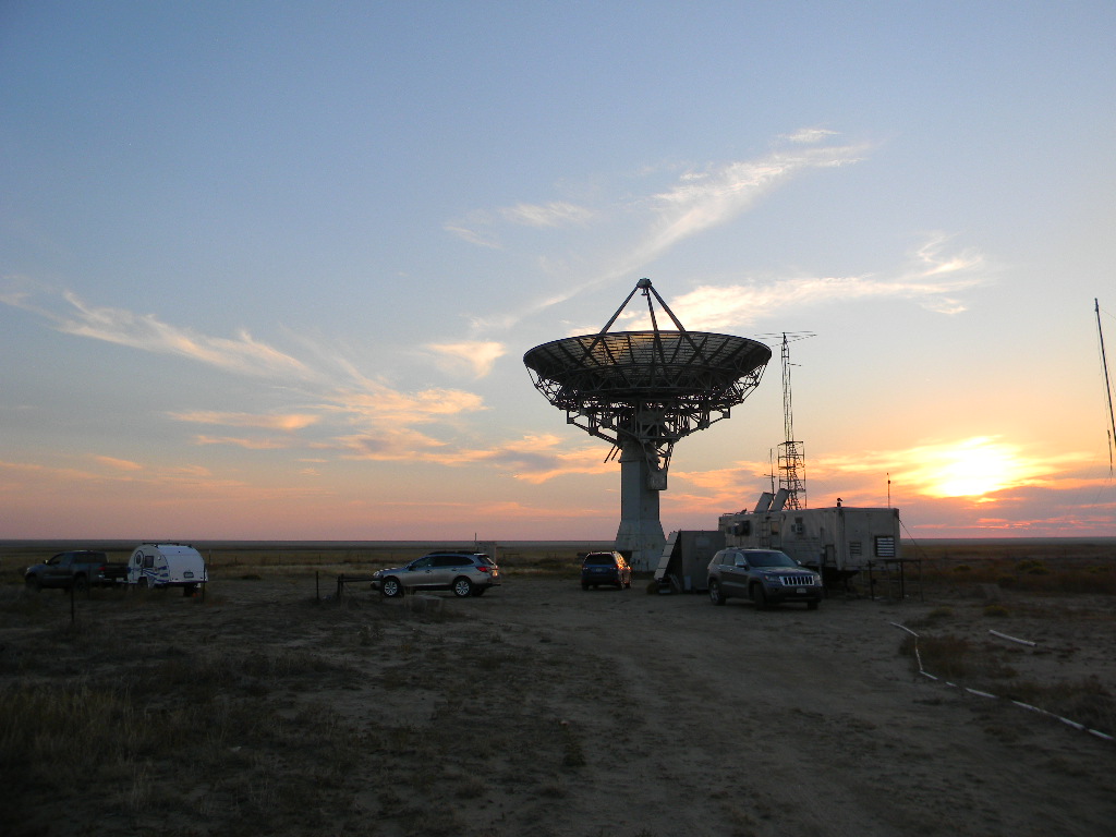
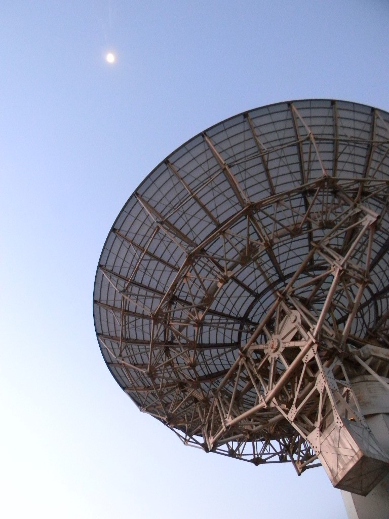
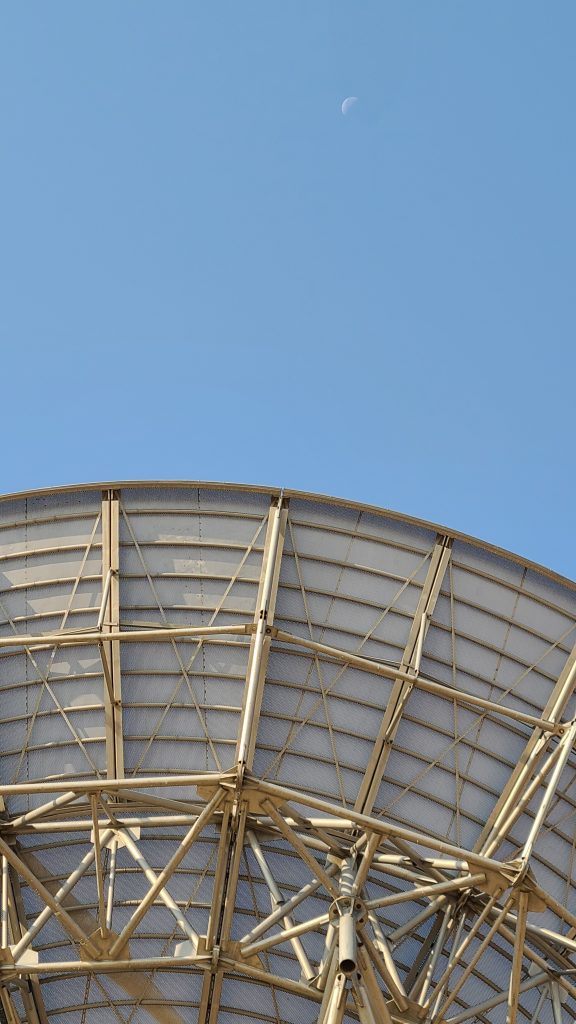
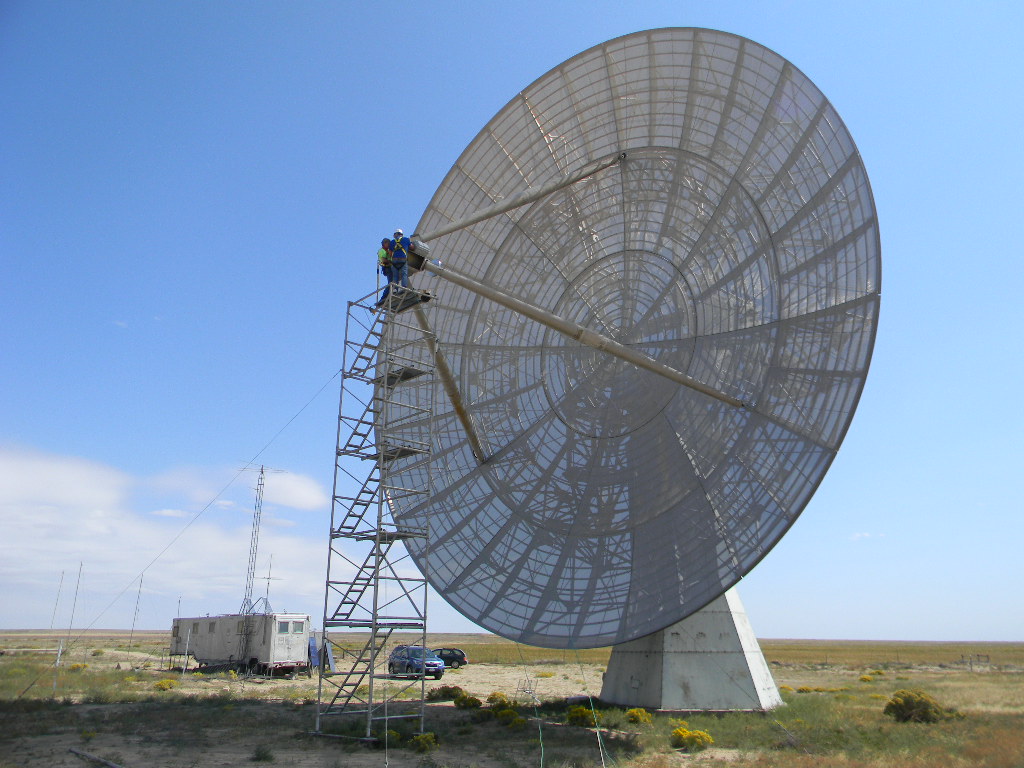
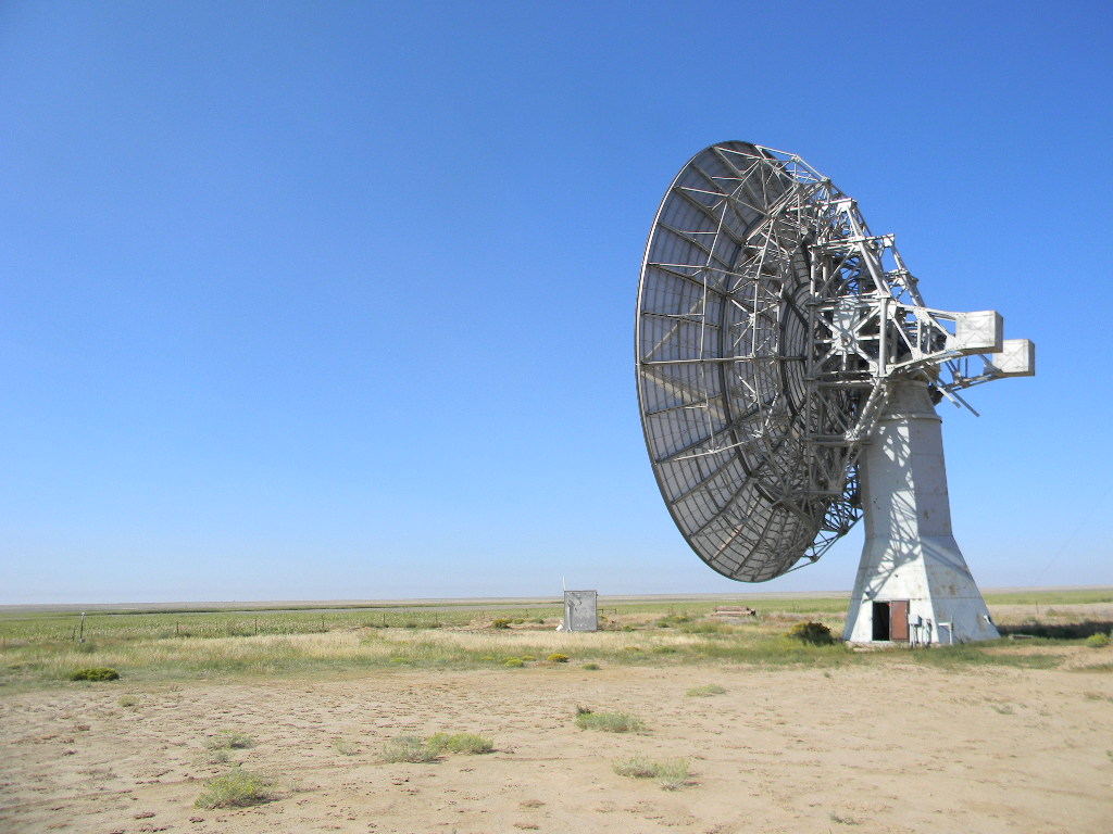
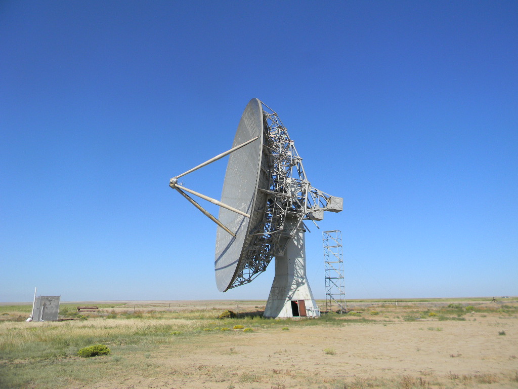
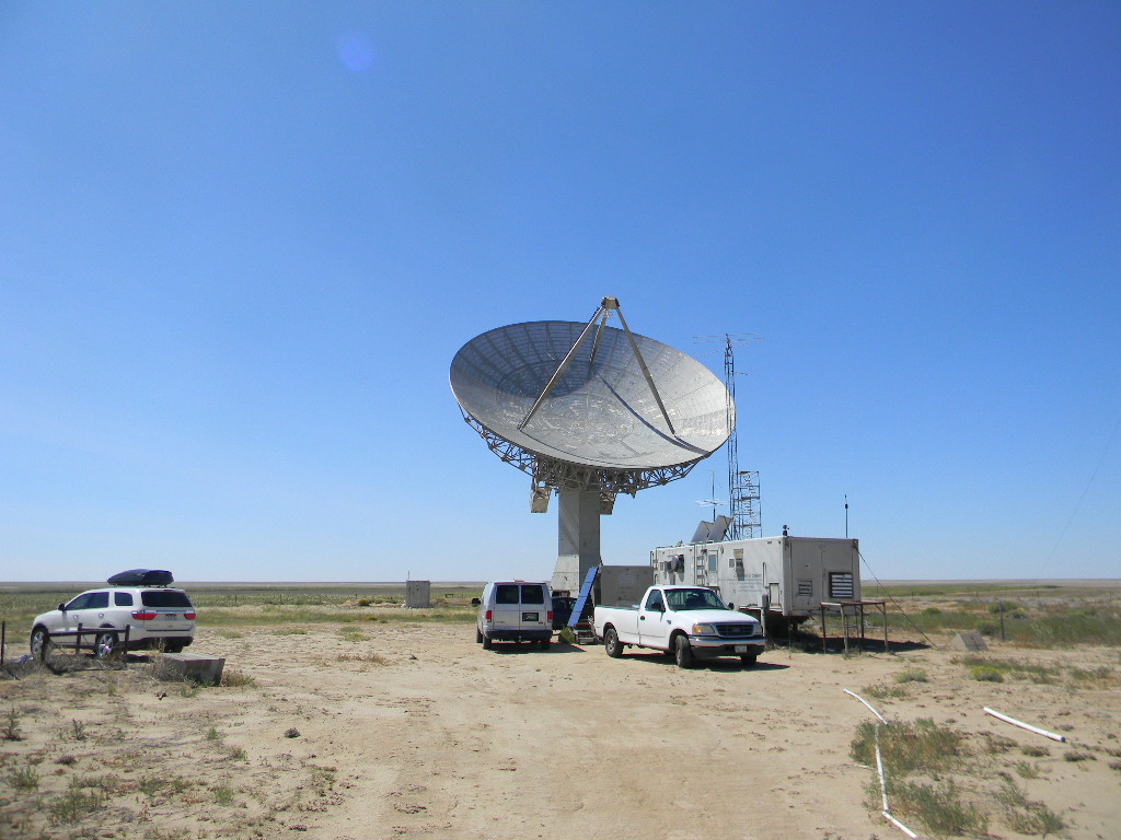
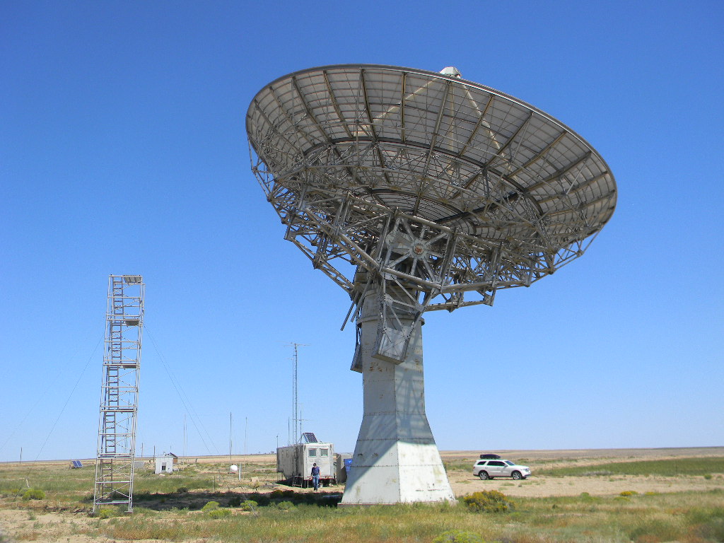
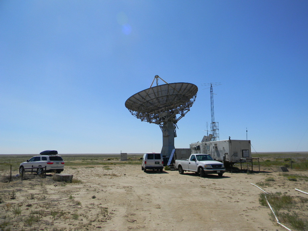
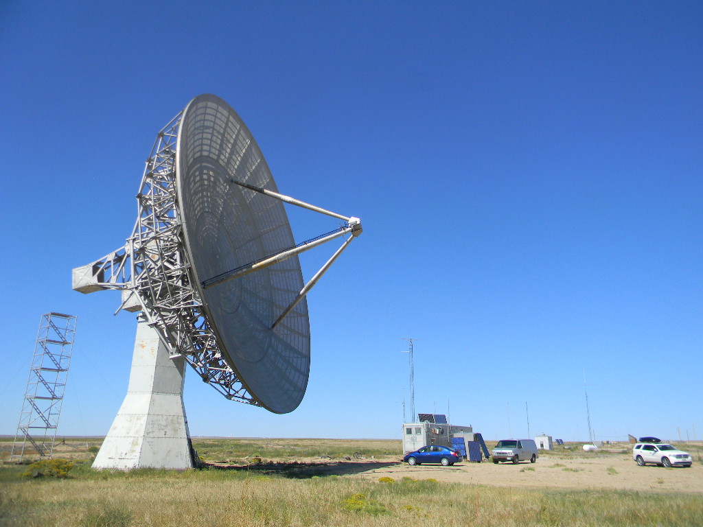
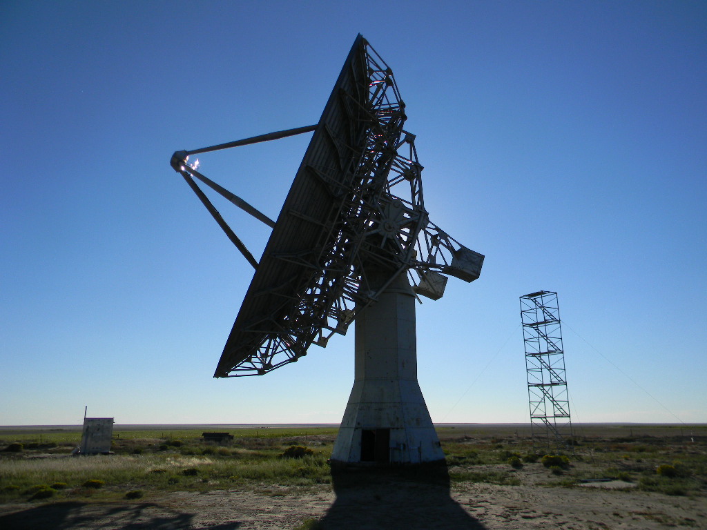
We did this participating in the annual ARRL EME contest held on the weekend of October 10-11, 2020 GMT. (That’s Friday 6 pm to Sunday 6 pm local time.) The frequencies available for this contest were in the ham radio bands from 50 to 1296 MHz. We used our 60-foot dish antenna at Haswell, CO, with a 1296 MHz feed with dual circular polarization, installed 2 weekends earlier.
EME Moon Bounce communications is directing a signal to the Moon. The Moon’s surface simply reflects the signal back to Earth. If the Moon is above your horizon, if you have suitable equipment, and if you know enough about what to do, it would be possible for you to receive the signal and communicate back. You could communicate to your neighbor or across continents. The signals, however, are extremely weak, having to travel back and forth the Earth-Moon distance, over 238,000 miles. EME generally requires efficient directional antennas to sufficiently increase the signal gain. Amplifiers can be used too. And the antennas have to point to the Moon. Also, radio signals sent through the ionosphere experience a rotation in their polarization. And there is some effective rotation from other causes, including from the changes in orientation from the Moon and from operating on different points of the Earth’s globe. Our solution is to circularly polarize our signals. And also, there is a Doppler shift between transmitted and received signal, mostly due to the Earth’s rotation, causing a difference in velocity between the Moon and our location on Earth. All of these are challenges to deal with.
Our 60-foot dish antenna at sunset as we started preparations. Photo by Glenn Davis.
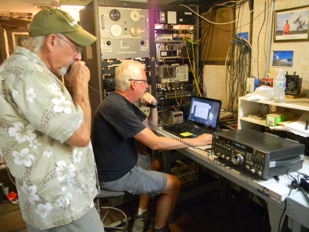
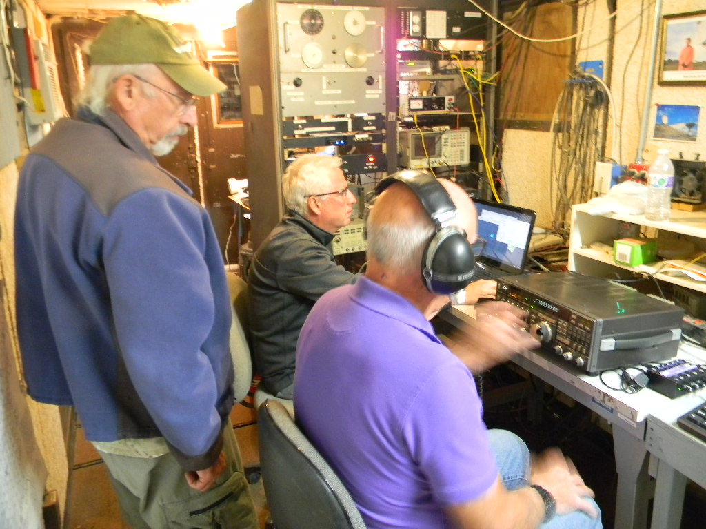
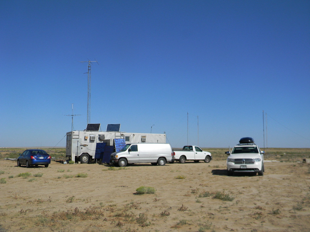
Our team for the EME operation were Ray Uberecken AA0L, Myron Babcock KL7YY, Gary Agranat WA2JQZ, and Glenn Davis. Bill Miller KC0FHN also came on Saturday morning.
The team arrived Friday evening October 9, while we still had daylight, to set up and test. Testing included making pre-arranged tropospheric scatter contacts, which were successful. We also attempted to complete set-up of a Hughes Internet antenna, to give us Internet access, but that was not successful. We instead sometimes connected to the Internet using cellphones. Although the contest began at 6 PM local time, we had to wait for the moon to rise above the horizon. Moonrise for us was at about 11:30 PM local time, and the Moon was above our horizon until about 2 PM local time the next day Saturday. We chose to stay for just this one Moon pass, and not continue through Sunday, in order to not knock ourselves out on this first attempt.
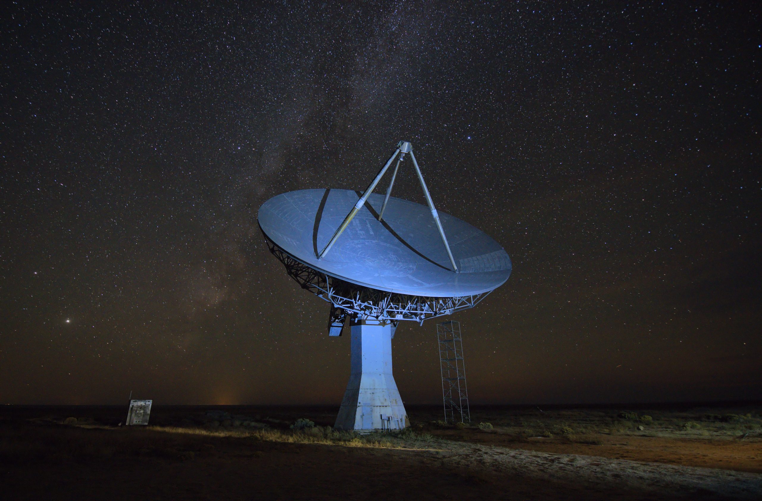
After we completed our testing, we relaxed until we were ready to start. Looking outside, we had an exceptionally deep starry sky. We could see the Milky Way clearly arching overhead through Cygnus. Jupiter and Saturn were bright to the south, and Mars was very bright, rising in the east. Glenn Davis experimented with his camera and took some nice time exposure photos with the dish antenna, the stars, and the Milky Way.
Photo by Glenn Davis. (Click to enlarge.)Our 60-foot dish antenna with the Milky Way. Jupiter and Saturn are brightly visible to the left of the antenna. Photo by Glenn Davis. (Click to enlarge.)
I (Gary) meanwhile got some rest. This enabled the others to get some rest later in the morning while I continued.
Myron KL7YY wrote and emailed an update about our operations to the DSES membership on Saturday morning at around 4 AM. It provides a good narrative of how we were doing until that point, and his update follows next:
* * * * * * * * * * *
Summary of DSES first attempt at EME, Earth Moon Earth, contacts using the 60 foot dish:
On Friday evening, October 9 we started with a few nearby Tropospheric Scatter contacts around 7 PM with DSES member KL7IZW, Steve in Monument, CO, and W6OAL Dave in Parker. Around 9 PM we talked to N0YK in Scott City KS, These contacts ranged from 110 to 130 miles and confirmed that our system was working.
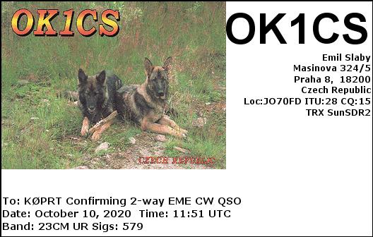
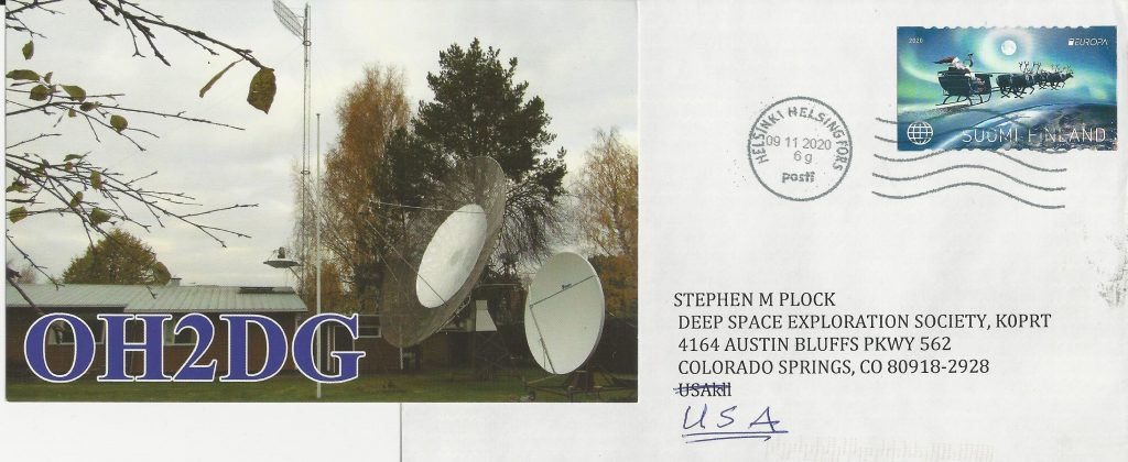
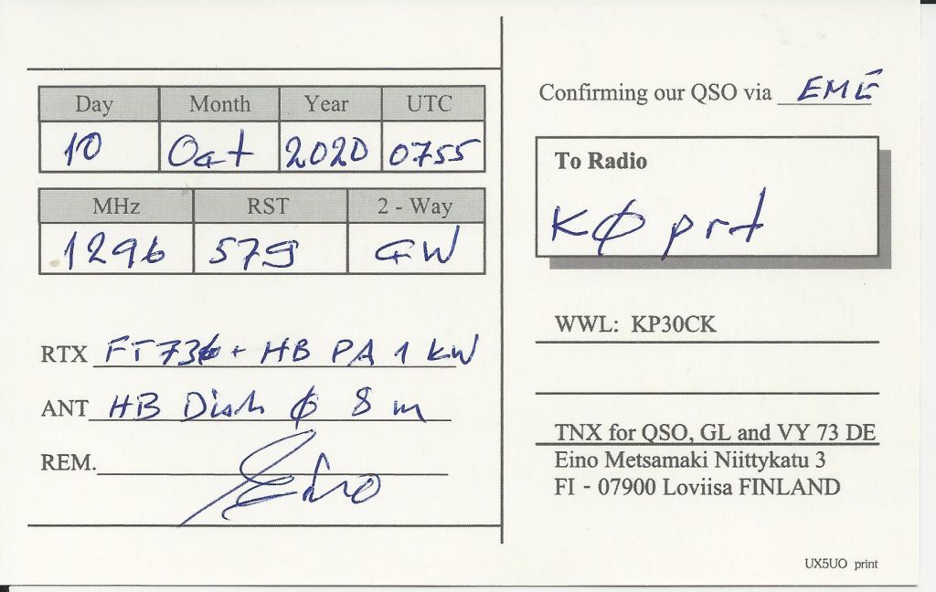
When the moon came over the horizon at midnight we tried to listen to the ON0EME moon beacon in Belgium but couldn’t hear it. About 45 minutes after moon rise we started to hear JT-65 digital signals. 10-15 minutes we started to hear CW signals. Glenn Davis made a few corrections to the tracking program and signals increased in strength. At times it sounded like a 20 meter CW contest pileup with all the loud signals bouncing off the moon all across 100 KHz of band (1296.0 to 1296.1 MHz). After about 90 minutes without hearing our own signal we rechecked the power to the amplifier at the feed horn and everything appeared to be normal. A few moments later we finally heard our own signal 2.5 seconds later on CW off the moon and the Belgium Moon Beacon. I made several calls on SSB and heard our echo really loud. We went back to CW and Gary proceeded to start making CW contacts. The first almost contact, a German station, abruptly dropped out so no official contact was completed. Our first official station worked on CW was with OH2DG in Finland. England was next followed by Italy, Poland, Denmark, Sweden and with DSES member Skip Macaulay, VE6BGT, in Alberta Canada.. Also made our first voice SSB contact with him as well. Seems that with every new contact we make it is with a new European country. In order to correct for Doppler shift and with no RIT we are changing VFO’s from Receive to Transmit by several KHz or more. Lots of CW signals being heard and we still have 12 more hours of moon to bounce signals off of… We are hearing our own echo and we have lots of hours to go. We plan on Digital mode later in the day but for now there are more than enough signals to hear on CW.
Our Moon bounce station consist of an older Yaesu FT-736R with 10 watts feeding almost 180 feet of half inch hardline into a 200 watt amplifier at the antenna feed horn. The receiver pre amplifier is a 30+db gain with a noise figure of minus .35. Our Effective Radiated Power (ERP) is over 6 million watts.
* * * * * * * * * * *
We operated with our club call sign K0PRT.
A short video of Myron KL7YY calling CQ. You can hear the echo of his signal coming back from the Moon a couple of seconds later. (Video length 35 seconds)
Because the signals are extremely weak, and there can be fading, there is a standard protocol for exchanging messages for EME contacts. This is intended to ensure as much of the message as possible can be copied and acknowledged on both sides. The basic format is simple, and one repeats a lot. One first exchanges call signs, then the signal reports, and then finally if that worked, an acknowledgement all that was copied correctly. If one only completes part of the contact, one should still log that, as that is an accomplishment. If using Morse Code, the standard is to send at 15 words per minute, but spacing out the characters longer than usual. The faster sending and spacing is to help one copy complete characters if there is fading. If one misses a character, one still has a high chance to get the character with the many repeats.
In order to have the proper frequency offset for the Doppler shift, we referenced the WSJT 10.0 software, at the suggestion of Steve KL7IZW. The software has an astronomical data section that calculates and displays the frequency offset. The higher the frequency, the more significant the offset. At 1296 MHz we had a difference of as much as 3 KHz between transmit and receive frequencies. The software also displays other useful data like local Moon rise and set times (based on Grid Square location).
The WSJT 10.0 software also can be used for JT65C digital EME communication. However, we didn’t figure out how to configure that in time with our setup, and so we didn’t do any digital contacts this time. We could tell we were hearing JT65 signals. They were present from 1296.05 to 1296.1 MHz, and we almost always could hear those signals while the Moon was up.
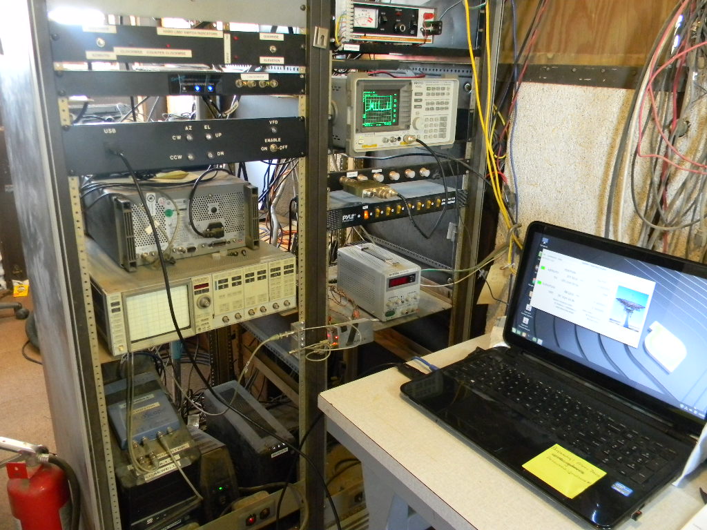
Glenn stayed up until about 3 AM, when we were sure our antenna azimuth alignment was correct and would continue to point accurately to the Moon. His work was invaluable in troubleshooting the azimuth offset, which turned out to be about 1.5 degrees, and honing in on the Moon once we heard CW signals.
Glenn Davis working with the antenna pointing. Photo by Gary Agranat.The 60-foot antenna pointing east, for the tropospheric scatter test to N0YC in Kansas. Later we would point east again, to prepare for where the Moon would rise. Photo by Gary Agranat.Myron making a tropospheric scatter SSB phone contact during testing, with Glenn Davis setting the antenna pointing. The scene was similar when me made SSB phone contacts during the EME contest. Photo by Gary Agranat.Myron, Glenn, and Ray. Ray was looking for the ON0EME beacon after the Moon rose. Photo by Gary Agranat.
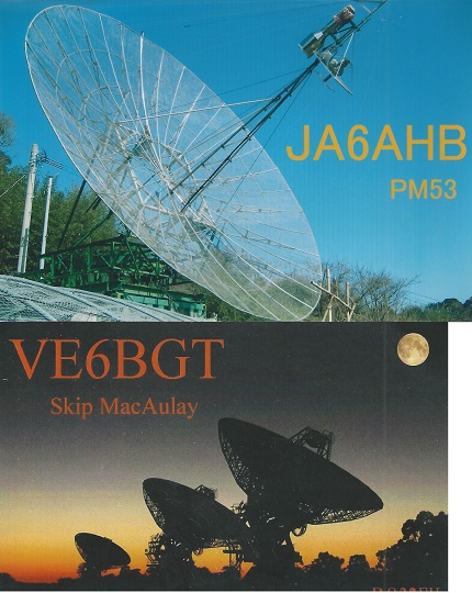
Since the Moon rises in the east, our signal paths at first are to the east. That is to Europe and the North American east coast. As Myron mentions, once we started receiving the signals, we were hearing many European stations, and we were busy. Through the morning we made 14 contacts to Europe, to 8 European countries. We also made the contact to our DSES member Skip Macaulay VE6BGT in Alberta, Canada, on CW and then phone. W4OP in North Carolina, hearing us on SSB, then gave us a call on SSB too.
Ray AAOL brought a CW keyer that can send Morse Code with either a keyer paddle or a keyboard. It can store pre-programmed messages, like a CQ call. I (Gary) decided to use the keyer paddle, as that gave me more flexibility — I could quickly adjust for conditions — and I felt more comfortable as I am used to the key. Meanwhile, it seemed to me also that some of the CW contacts we made used software to send their messages. Those didn’t have good spacing between words or call signs. And that made copying slightly more challenging. A keyboard though can enable any of us to send, even if we don’t have practice sending Morse Code. Most of the contacts we made were with CW Morse Code.
This short video shows part of a Morse Code CW contact by Gary WA2JQZ. XE1XA in Mexico called CQ. We responded by sending our call sign K0PRT several times. Then K (the invitation to respond) several times. When we switch the VFO from the transmit to the receive frequency, you can hear the last part of our signal coming back, reflecting from the Moon, several seconds later. You then here the signal from XE1XA, also coming back reflecting from the Moon. He transmitted back our call sign as K0PRN, instead of K0PRT. We afterwards replied sending our callsign again, only, to give him the correction. That’s why we repeat a lot, and send sections of the message just one at a time. We completed the contact successfully. If you look carefully on the transceiver, you will see we switched about 2 KHz down from the transmit to receive frequency. (Video length 1:16)
At around 6 AM, when the Moon was high enough so that we no longer had a path to Europe, we took a break for breakfast and to rest.
Just before sunrise. Photo by Gary Agranat.Tracking the Moon during early morning. Photo by Gary Agranat.
In earlier discussions we thought we might have many more contacts across the Pacific and to the North American west coast, when the Moon was sufficiently to the west. But it turned out we had very few contacts that way. We made just two contacts to Japan. Our first was at about 9 AM local time, to JH1KRC. Our second was three hours later to JA6AHB. Instead we made a few more contacts to the US, a few to Canada, and one to Mexico. These other stations we heard were searching around too. That led me to believe that if there were any other signals out there, we likely would have heard them.
W5LUA Albert Ward in TX, who some in our group know for EME. (He at first thought I was Ray, when I contacted him on CW. Myron then contacted him on SSB.)
W6YX, the Stanford University radio club, which was using a 28 foot dish. We contacted them first on CW. Then later when Bill was looking to record a phone QSO, which would illustrate the signal delay from the transit time to the Moon and back, W6YX just happened to call CQ on SSB on the frequency we were tuned to. We then had about a 4 minute QSO on SSB with them, which Bill recorded.
A video of Gary WA2JQZ responding to W6YX at Stanford University and having a 4 minute SSB QSO. (Video length 4:38)
We operated until about noon. We made 30 contacts in all. 25 contacts were CW (Morse Code) and 5 were SSB phone. 4 of the 5 phone contacts were with stations we also had CW QSOs with.
We submitted our contest log to ARRL the next day.
In the judgement of all of us, we had a very good EME operation. We are very pleased it worked so well on the first attempt. We clearly have a capable EME station.
Glenn and his team are continuing to follow up to investigate why we had a 1.5 degree azimuth offset.
It still takes my breath away to hear the echo of our signal coming back from the Moon, a couple of seconds later. The speed of light isn’t just a value in the books, it is something you experience viscerally first hand. It is real. EME is the longest signal path we have for communicating with others. This is fun.
These are the contacts we made. (CW = Morse Code, PH = SSB phone. Given also are the date and GMT times, the signal reports, and the other stations and their locations):
Total Contacts by State \ Province: AB 4, CA 2, TX 2, BC 1, FL 1, NC 1, NJ 1, WI 1. 8 total.
Total Contacts by Country: USA 8, Canada 5, Czech Republic 3, Federal Republic of Germany 3, Italy 2, Japan, 2, Austria 1, Denmark 1, England 1, Finland 1, Mexico 1, Poland 1, Sweden 1. Total countries 13.
Total Contacts by Continent: Europe 14, North America 14, Asia 2. Total continents 3.
Cool Science Festival Presentation on Saturday October 11, 2020
Rich Russel made an online presentation at the Cool Science Festival. The presentation covered the science of radio astronomy and the accomplishments of the Deep Space Exploration Society. The presentation was streamed live on Facebook and Youtube. You can watch the presentation here:
Astronomer Rich Russel from the Deep Space Exploration Society describes how he uses the 60-foot Plishner radio astronomy dish antenna 90 miles southwest of Colorado Springs to detect pulsars in deep space.This live-stream presentation was part of our virtual Cool Science Carnival Day for kids, the main event of the 2020 Colorado Springs Cool Science Festival. You can find more information at:https://www.coolscience.org/carnivalday.html
This 8-day regional event, designed to ignite wonder and inspire curiosity about the world around us, attracts between 10,000 and 20,000 attendees each year. For more information about the Cool Science Festival go to:
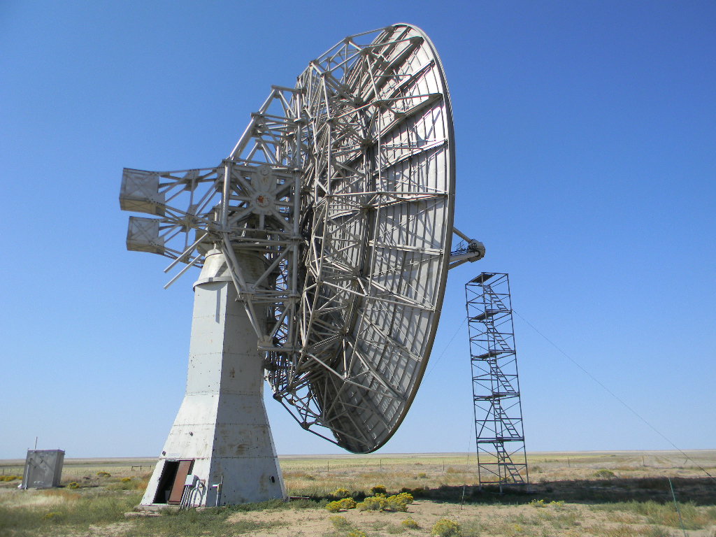
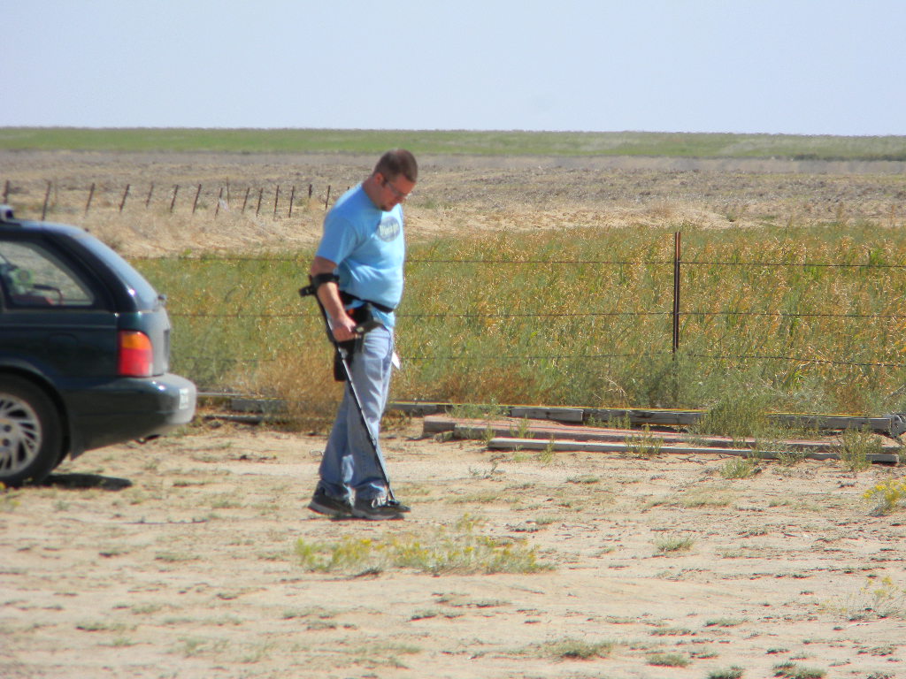
A DSES team worked at the Plishner Radio Telescope site in Haswell on Sunday September 27, 2o2o. Team members were Ray Uberecken, Floyd Glick, and Gary Agranat. We accomplished the main objective, to install a new 1296 MHz feed at the focus of the 60 dish antenna. We also installed a mast in the ground, on which will later be added a Hughes Internet satellite antenna. Two friends of Ray’s came out and did an immense service by using metal detectors and magnetic rollers to clear nails and other metallic debris on the site. We changed out two of the locks. And we inspected the bunker.
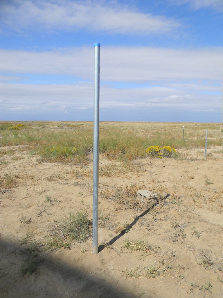
Mast for Hughes Internet antenna
Ray and I met at the Plishner site at 0930 in the morning.
We first installed a sturdy pipe mast behind the operations trailer, on which will be mounted a small satellite antenna to access the Hughes network geosynchronous satellite for Internet access. Ray chose a spot that will not be blocked by the trailer or the 60-foot antenna. We mixed cement and set the pole in its hole with the cement, using a level to check that the mast is vertical.
Moon Bounce (EME) Preparation
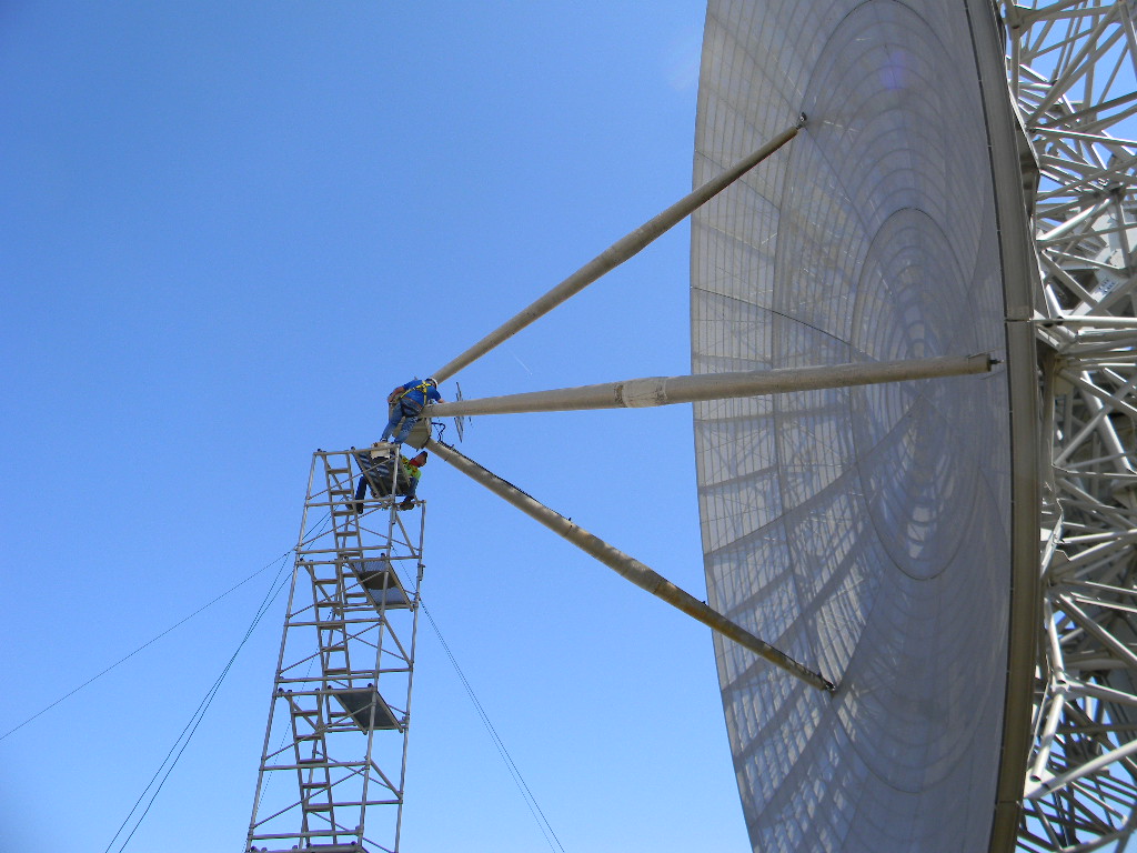
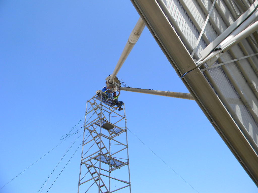
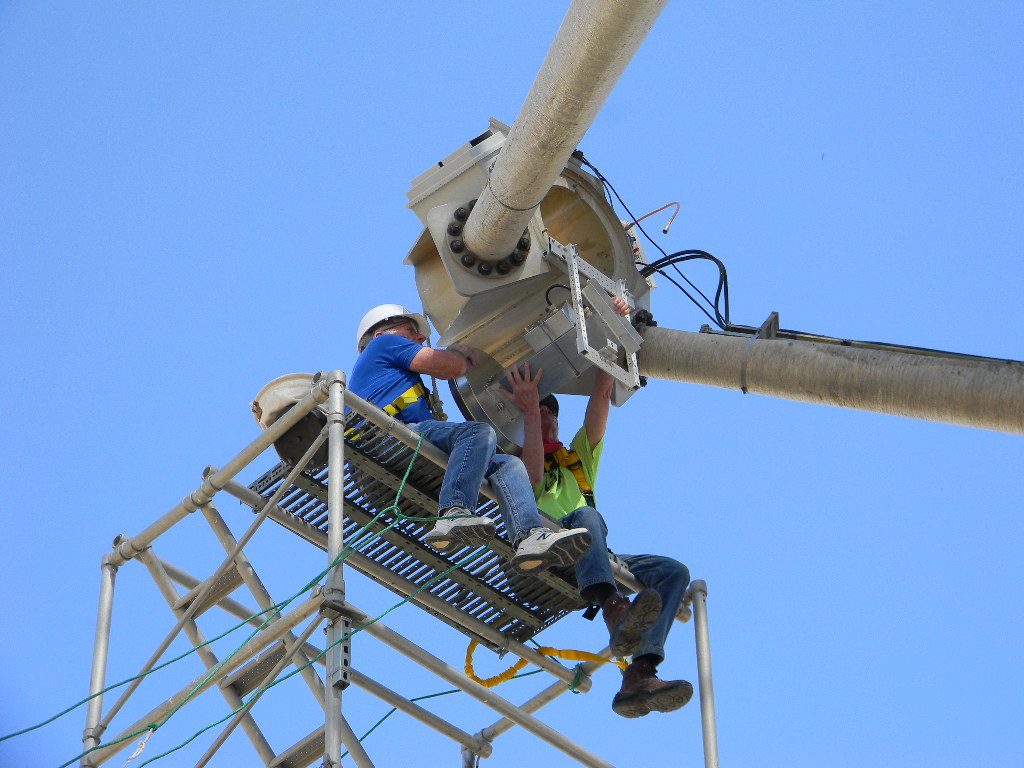
After that we manually rotated the 60-foot dish antenna to the service platform. I figured out, with Ray’s help and the checklists, how to use the software to monitor the antenna pointing. (Note: we might want to add a checklist just for this type of procedure, for using the software for just manual antenna pointing, as when we service the antenna.)
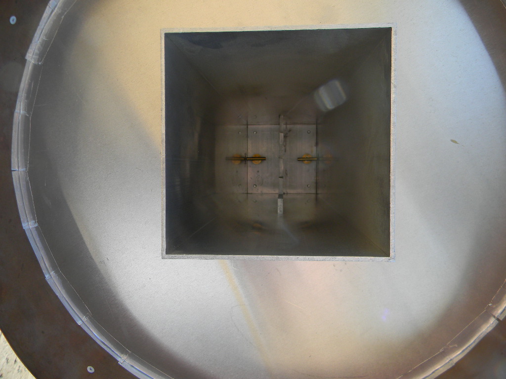
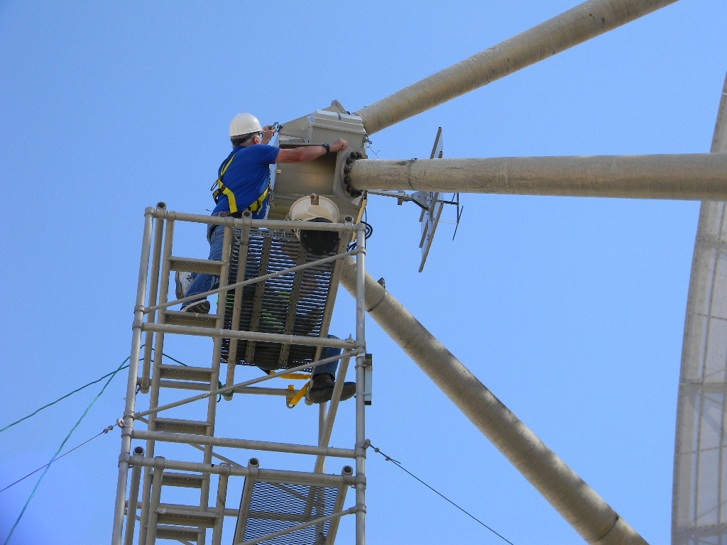
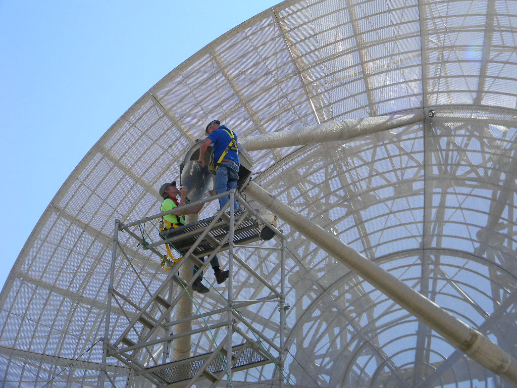
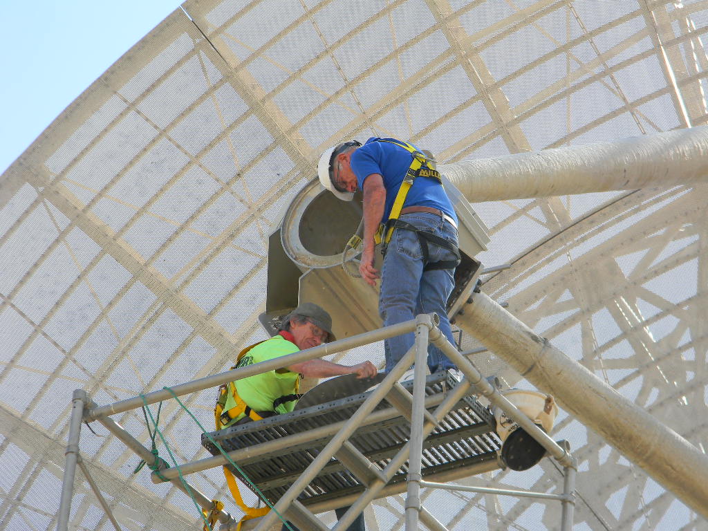
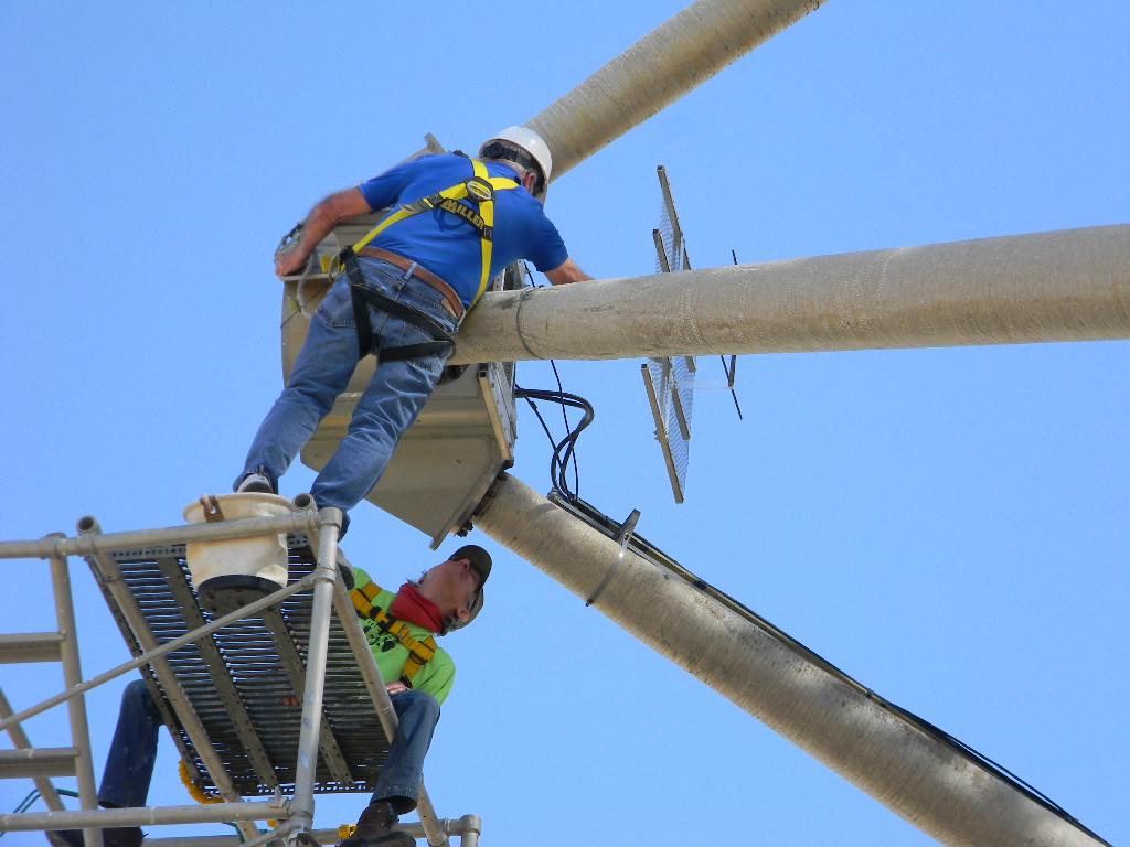
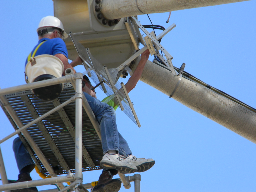
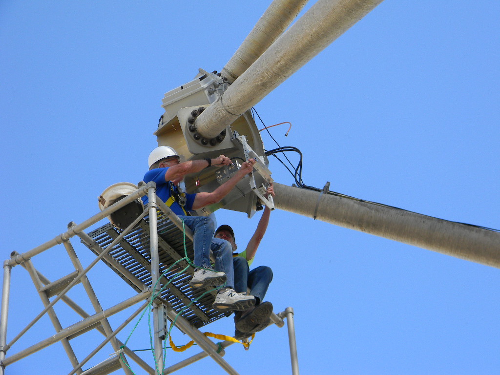
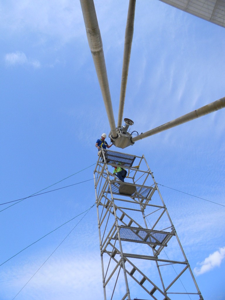
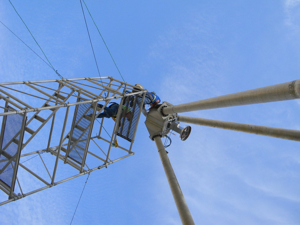
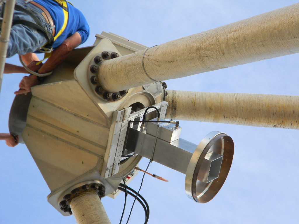
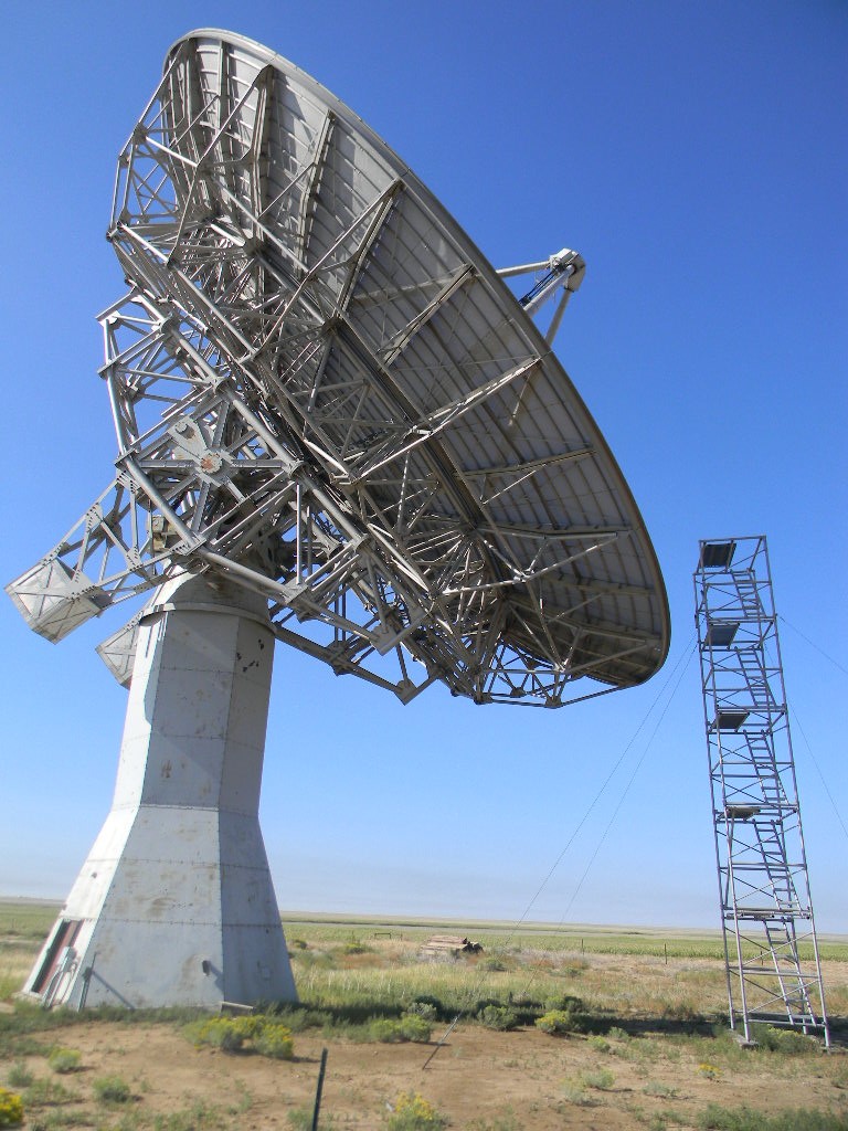
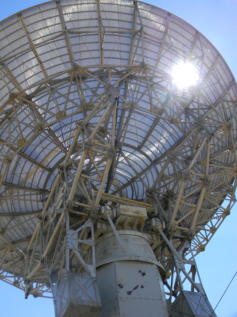
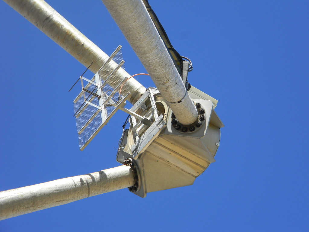
Floyd came out to the site by 1030. Ray and Floyd climbed the service platform. I worked on the ground to move feeds and tools up and down to them. We replaced the 408 MHz feed at the antenna focus with the newly built 1296 MHz feed. The 1296 MHz feed was built by KL6M, to specifications provided by Steve Plock (KL7IZW). The feed mount at the dish focus was designed by Ray, to enable the feed to more easily rotate out and be changed.
Conditions were somewhat windy, with a cold front coming, but still manageable. By the afternoon the winds had picked up enough that we postponed any further work at the feed. Work that still needs completion is installation of a 200 Watt amplifier at the feed. Since we are planning to operate at 1296 MHz from the Operations Trailer, which has a long coax hard line path to the pedestal and antenna feed, we expect significant power loss from the long path. We therefore need to boost the power again at the feed. We plan to install the amplifier the next weekend. We then also intend to test our setup by trying tropospheric scatter communications to the north.
We are planning to use this configuration to operate EME (Earth Moon Earth) Moon Bounce communications. And specifically we plan to participate in the ARRL EME contests on October 10-11, 2020 and on November 28-29, 2020 (UTC).
We discussed our plans for the upcoming contest in 2 weekends. The Moon then will be at last quarter phase. What that means is that it will rise on Friday night a little before midnight (about 1130 PM), and set Saturday a little after 2 PM. That means we will prepare to do overnight and morning operations. After the Moon rises we will try to pick up the ON0EME beacon in Belgium. We can try to contact across the Atlantic Ocean. The US East Coast will be in night time conditions, and so we anticipate less contacts to there. Daytime conditions, when more hams would be awake, are more favorable for the US West Coast, and across the Pacific Ocean to Oceana, Asia, and Australia.
Note that the 60-foot antenna will be configured with the 1296 MHz feed through the end of November. This will be an opportunity to try using it for other 1296 MHz communications, including troposphere scatter.
Metal souring of the site
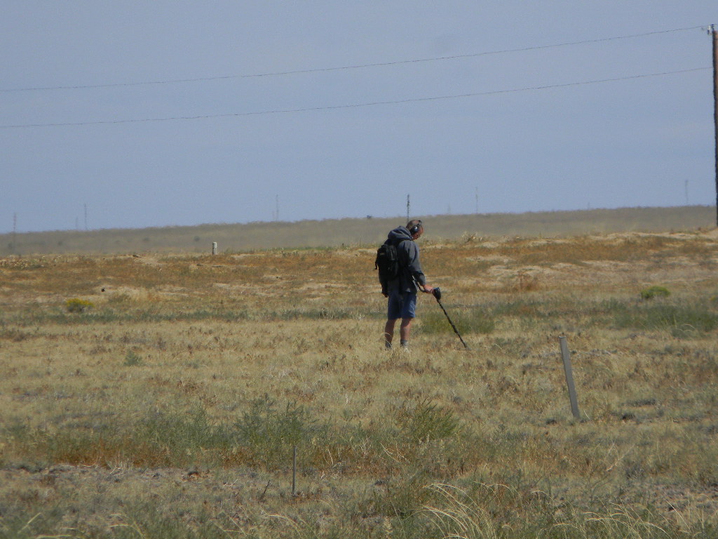
A friend of Ray’s who works at Planet Granite Ryan, and his brother, Rob, came out to the site also. They have ground metal detectors and magnets on rollers, and systematically paced across the site to pick up nails and other small metallic debris. They did pick up lots of nails, including along the roadway. They spent a few hours with us, and left after lunch. They did us a great service by helping remove a lot of this debris.
Combination Lock and Bunker Inspection
We attempted to open the combination locks at the gate, the bunker, and the generator shack. After still having difficulty, we replaced the locks at the gate and bunker, with the locks Myron Babcock obtained for us. These are similar model locks, and the combinations were kept the same.
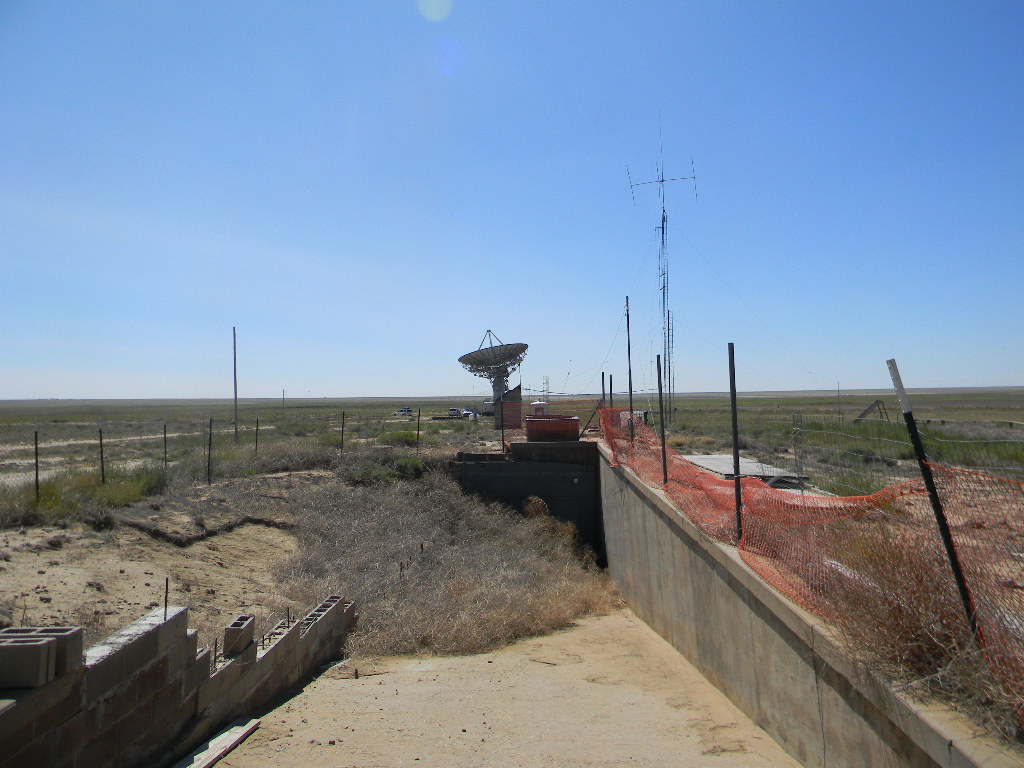
We had a report that the bunker had been flooded by two successive rain storms in July. We opened and inspected the bunker. The bunker was dry, though the floor had more-than-normal dust and dirt, and some tiny debris was spread here and there. It will require a fresh cleanup before normal use. We saw no indication of mold from dampness.
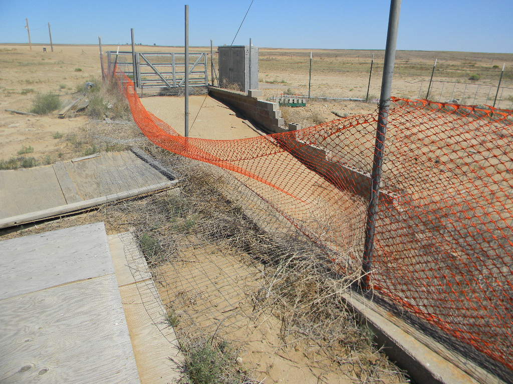
Tumbleweeds were accumulated again at the ramp entrance.
We completed our activities by early afternoon, about 3 PM.
For the team, – Gary
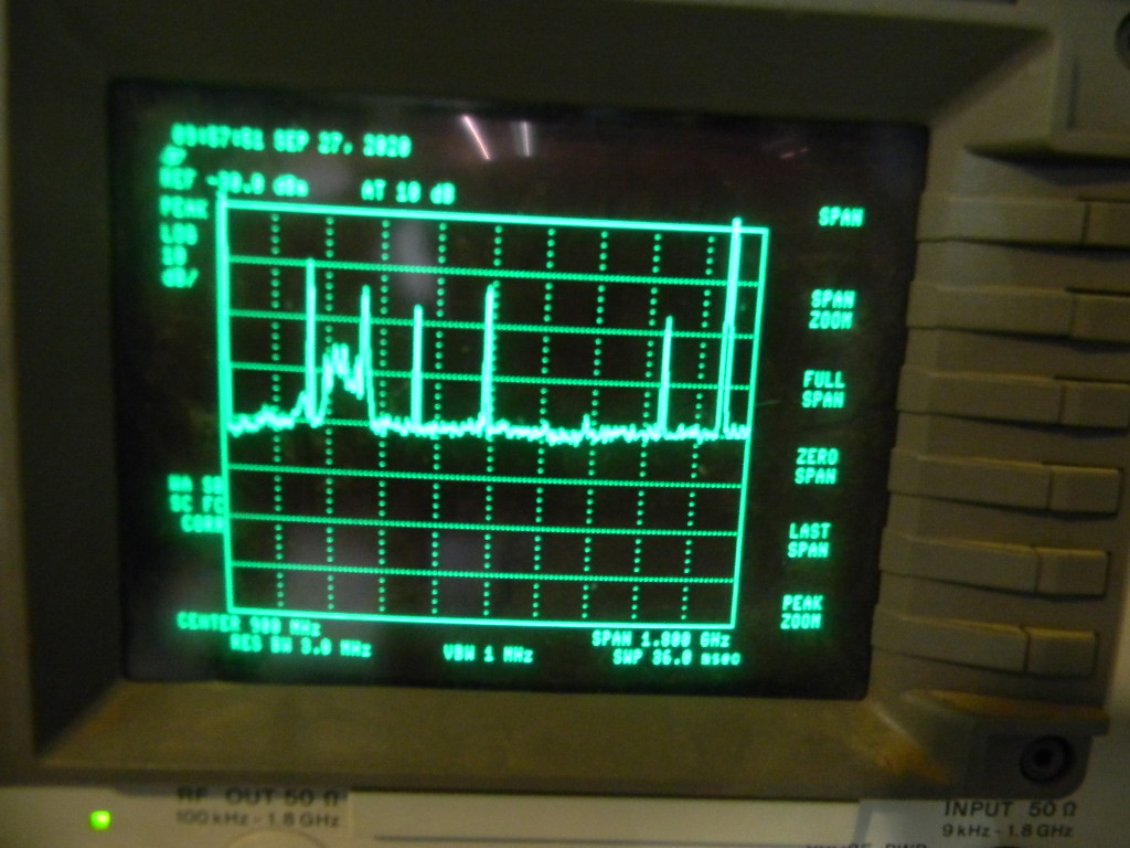
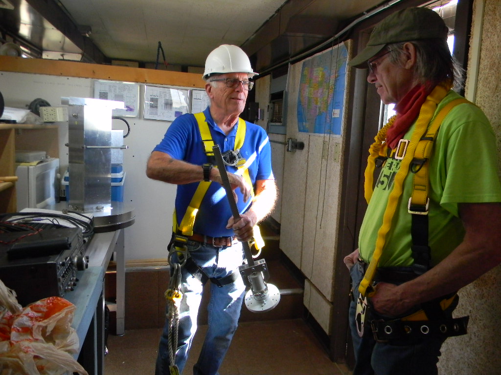
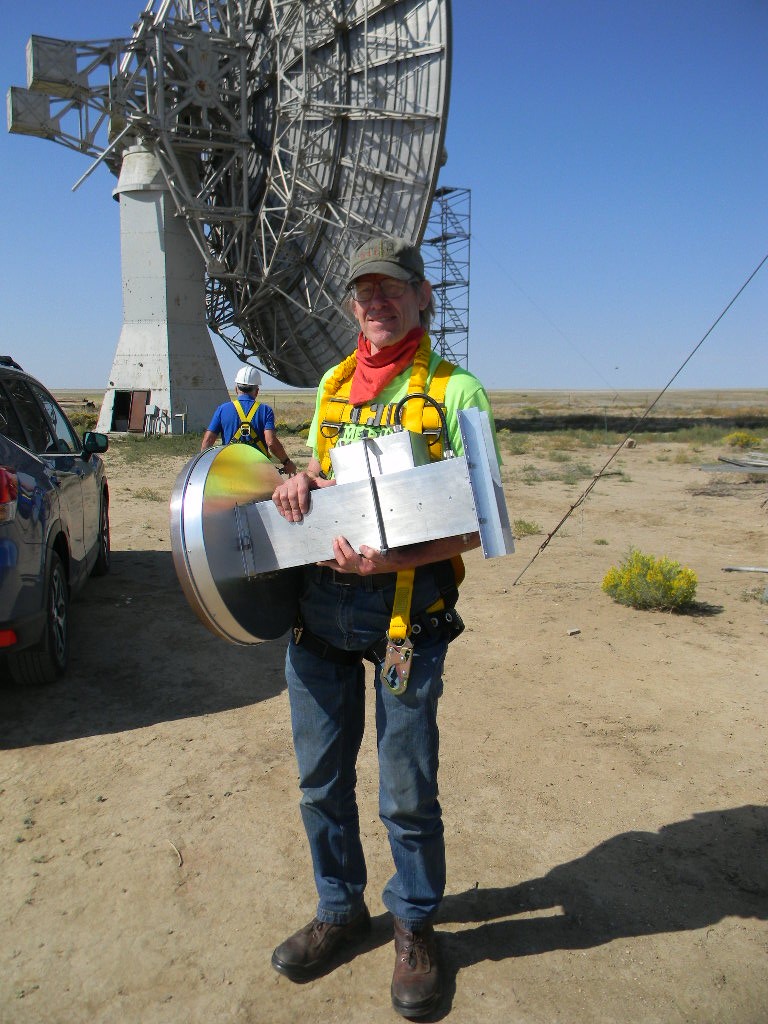
We kept the antenna steering in manual configuration. We opened the System 1 steering software to monitor the position angles as we manually steered the antenna to the service platform.We noted this radio interference at the site on our scope. This scan is from 0 to 1.8 GHz. The higher floor noise level at the left is from the sensitivity of our 408 MHz feed, which was still on the dish antenna, before we changed it out.The 60-foot antenna is positioned for service.Ray brought two feeds for the 60-foot antenna. This is Ray showing Floyd the 4 GHz feed, which we will use in the future, to calibrate the pointing position with geosynchronous satellites.Floyd carrying the 1296 MHz feed to the antenna for installation.The inside of the 1296 MHz feed. It is designed as a septum feed, with separate channels on each side for left and right circular polarization.Rob with a metal detector, crisscrossing the site, picking up small metal debris.Ray and Floyd on the 60-foot antenna service platform, starting work.Removing the cover.Ray is disconnecting the 408 MHz feed, so that it can rotate down and out for changeout.The 408 MHz feed is now rotated down. It is connected simply by the shaft to the mount, for easier changeout.Installing now the 1296 MHz feed. Its design doesn’t use a shaft, but instead will be securely fastened to the mounting frame.Ryan using a metal detector on the west side of the site.Our view towards the west. High clouds in the distance are an indication of a cold front gradually coming this way. We experienced steady windy conditions as the front approached..Closing up.Our view of Haswell in the distance. The clouds from the front were getting closer. By the time we left in mid-afternoon, the clouds were over us, but we had no precipitation.The 1296 MHz feed installed.We installed this ground mast. It will mount a small satellite antenna, to connect to the Hughes Internet network.
Text and photos by Gary Agranat. Analysis pdf by Rich Russel.
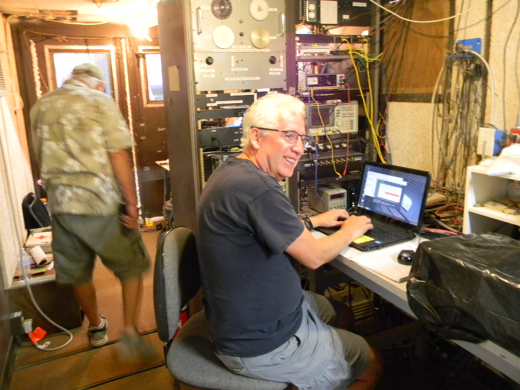
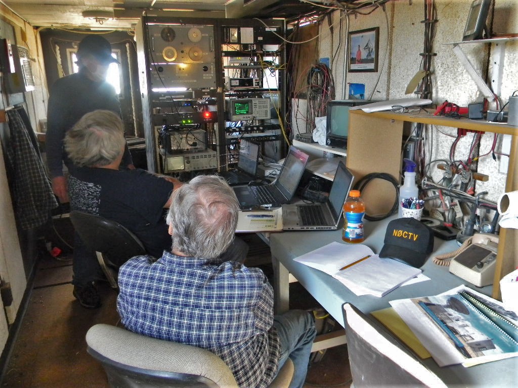
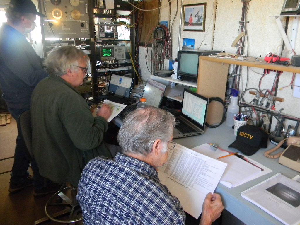
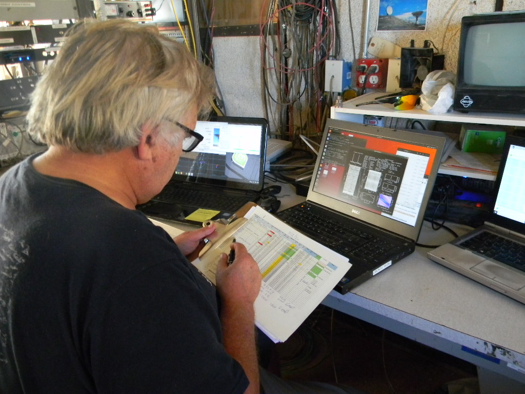
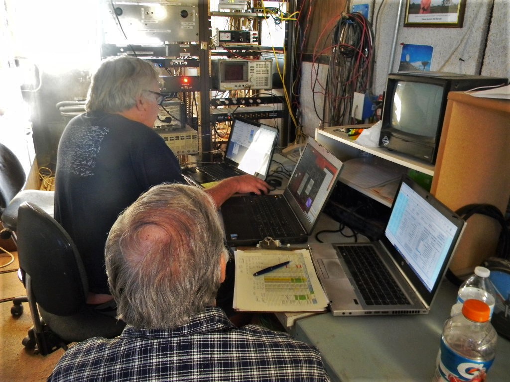
On Saturday September 12, 2020 an observing team of Rich Russel, Bob Haggart, Bill Miller, and Gary Agranat spent the day observing pulsars. This is the first observing session since we recalibrated the 60-foot antenna azimuth pointing the weekend before. The team observed 3 pulsars we had not seen before. Plus several other pulsars were attempted. The team spent the whole day at the site, from about 9 AM to 7 PM.
The pulsar signals are so faint that we cannot detect them directly. To observe them, we have to point to the correct celestial coordinates and then track that point as the Earth rotates. While we are pointed, our computer accumulates the signal data. We need at least a half hour continuously tracking the position. At this session some of our observing runs lasted 2 hours, for the fainter objects. At previous sessions we have tracked for as long as 4 hours.
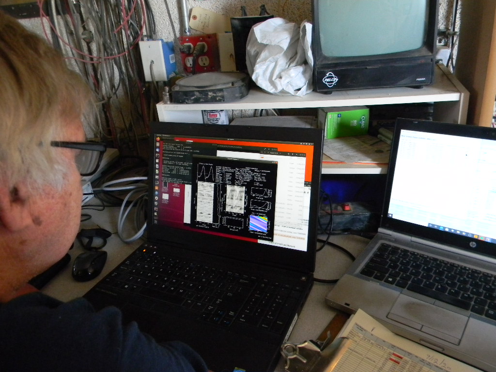
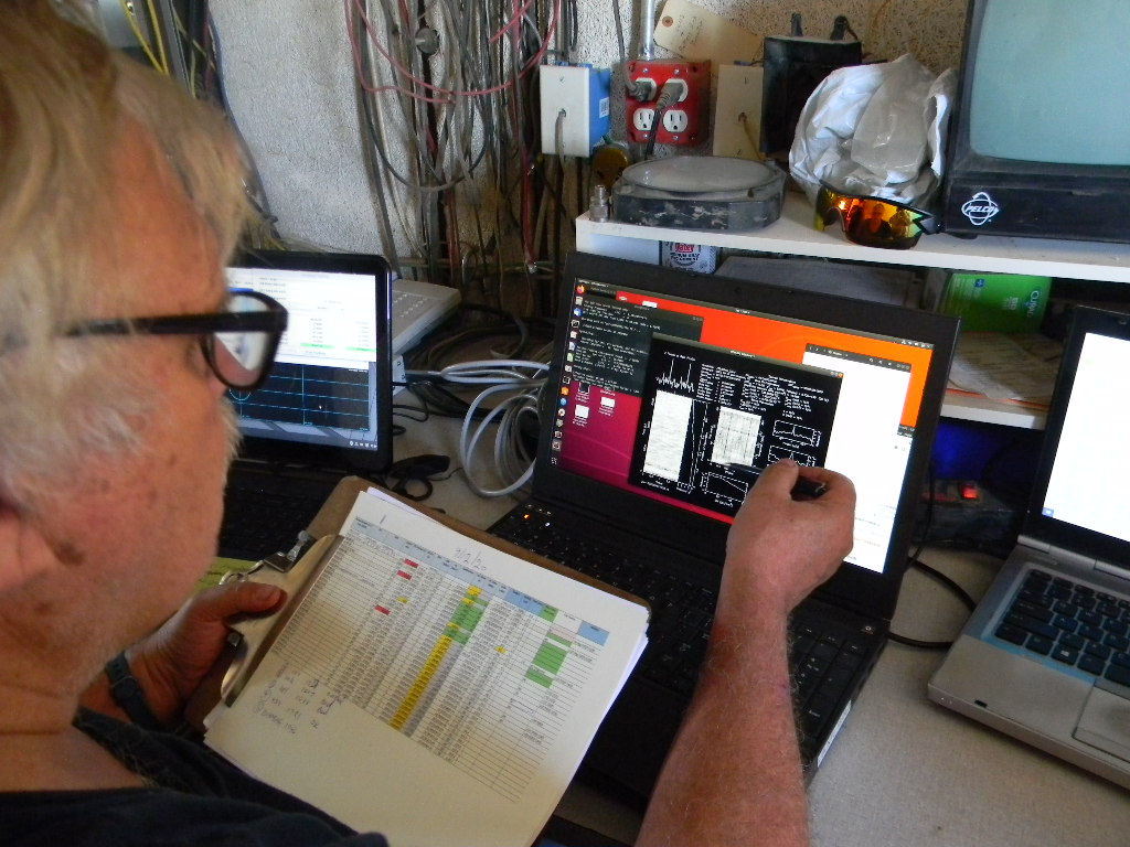
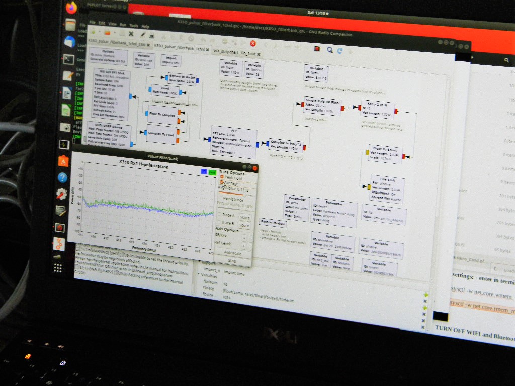
After the observing track, we have our software process the data. The random background noise should cancel itself out. But the pulse signals should build up with time. If we have the correct timing interval of the pulses, and if everything else is working, the computer display will show the pulses, and several other parameters.
Pulsars are very unusual objects. These are what remain of massive stars (greater than 5 solar masses) after they use up all their fuel for nuclear burning. These more massive stars fuse heavier and heavier elements at their cores until they start to fuse iron from silicon. Unlike the fusion of other elements, iron requires energy to fuse, rather than produce energy. The sudden reduction of energy at the core drops the temperature and pressure there. The pressure at the core is no longer enough to counter the weight of the star’s material above it. Gravity is now the stronger force, and the material above collapses in on the center. The pressure and temperature at the core then becomes even higher, which starts new reactions that fuse the matter at the center to neutrons, and and which also generates neutrinos. The outer layers falling in at great speed bounces back out. The result is a supernova explosion. What remains is the neutron star at the center. It is extremely massive and compact. And like an ice skater rotating faster as the arms are brought in, the star’s rotation speeds up immensely. The star’s magnetic field also has become compressed and much more intense. Charged particles will rotate around the magnetic field lines, with very high energy. Whenever charged particles are forced to deviate their paths from a straight line they emit electromagnetic energy, like visible light and radio. At the neutron star’s poles, this energy is channeled out, with immense energy. Because the magnetic poles are generally not at the same spots as the rotational poles, the beam of this light and radio is spun around like a light house. If Earth happens to be in the path of such a beam, we detect that as a pulsar. So that’s what we’re observing. These neutron stars are hundreds and thousands of light years away.
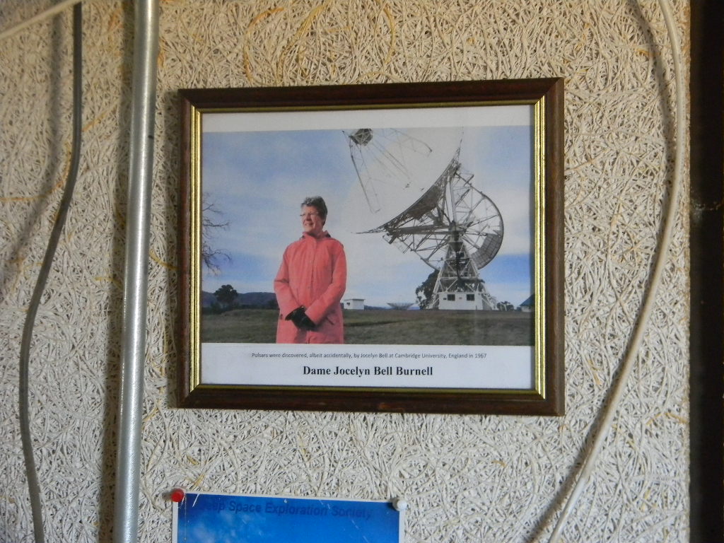
Pulsars were first discovered by accident in 1967, by Jocelyn Bell (now Jocelyn Bell Burnell) who was then a graduate student at Cambridge University. Bob contributed a recent photograph of her, posed by some radio telescopes. We now proudly have that displayed on the wall above our computer displays.
Because the observing runs take a while, for this session we decided to try watching some videos. Bob brought a DVD player and a large monitor. Gary brought some educational videos, including one about the Crab Nebula and pulsars. Rich brought some movies.
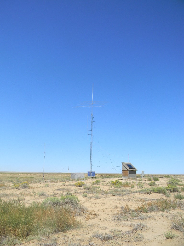
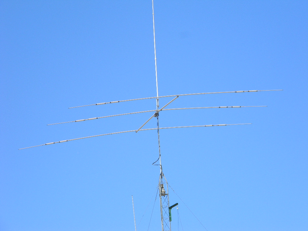
On this work trip the team also inspected damage to our ham radio antennas, damage probably from the storm weather over the past months. 7 radials at the base of the vertical antenna were damaged. And the 3 element Yagi antenna on tower was slightly tilted along its longitudinal boom.
Tumbleweeds also had accumulated again at the bunker ramp. Some of the surrounding fence had also been damaged from the weather. Rich Russel brought some fencing to use in the future, to place over the immediate entrance path to the bunker door.
Repair of the ham antennas and ramp clearing will be planned for a future work trip.
Below is a photo narrative of the day’s work.
It was an excellent day’s work.
At the start of observations, we point to and observe a pulsar with a strong signal that we know we should be able to reliably receive and analyze. If we cannot detect it, that indicates something is wrong with our system. We would then troubleshoot rather than waste our time trying to observe. Here the antenna is pointing to a pulsar we use as a reference source, B0329+54. It is located in the circumpolar sky to our north, so it is always visible above the horizon for us.Bill Miller, Rich Russel, and Bob Haggart starting observations in the Operations Trailer.After we checked our equipment and processes, we tried looking for some pulsars that were relatively low on the horizon to our south. Objects that appear to the south are above the horizon only briefly. They rise in the southeast, as the Earth turns they continue to rise in a shallow arc above the southern horizon, then soon set in the south west. If we want to try to observe them, we have just a short window of time to find and track them. Being low on the horizon adds some bias errors and attenuation to the observations. At this session we didn’t succeed in observing any pulsars that were close to the southern horizon.On this run, the display shows we did not get good data. The software is attempting to synchronize our data with an expected pulse period. In the top window display that is open, for good data we would expect to see clearly spiked peaks rising from a lower noise floor. And in the white rectangular box below that, we would expect to see a signal at that timing accumulate under such spikes. There is no pattern of periodic data. The white box to the right shows timing at the bottom with radio frequency at the side (going up). Because the pulsar signal is broad band (it is spread broadly over a wide range of frequencies), we would expect to see a continuous line of signal from bottom to top, across the frequencies. But we do not see that. (You can click this image to enlarge it.)
The two graphs in the center right tell us we don’t have a definitive measure of a pulse rate, and a steady change in pulse rate. The pulsars are generally slowing down with time, at a very slow but measurable pace. The display is showing the algorithms cannot fit a pattern. If it could, the two peaks would both be centered.Our Operations Trailer
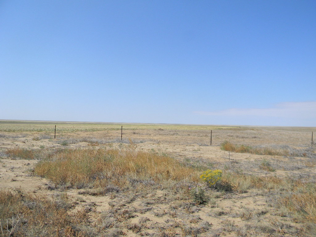
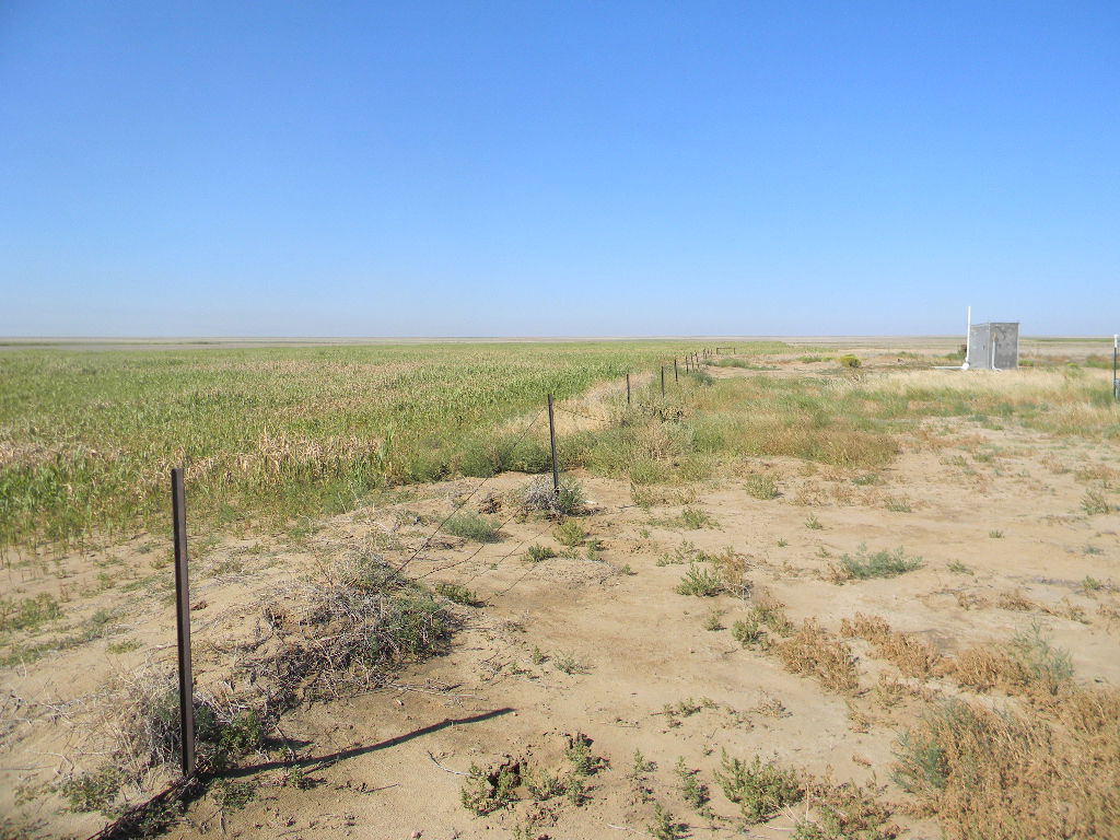
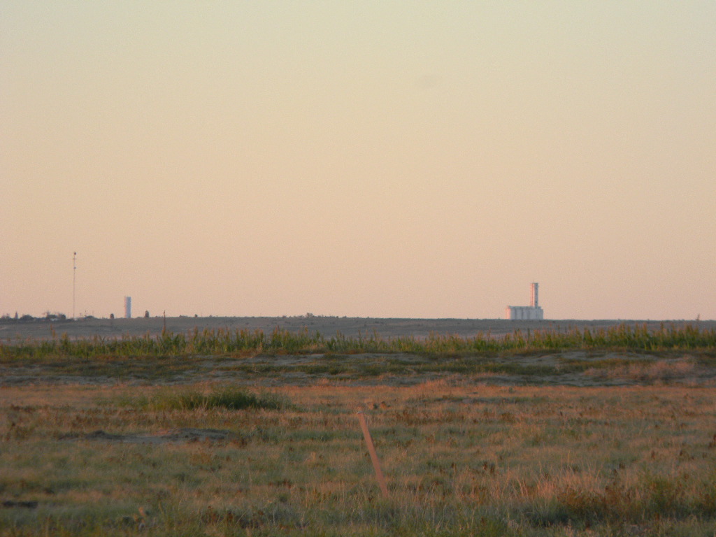
Our antenna site is surrounded by farm fields.
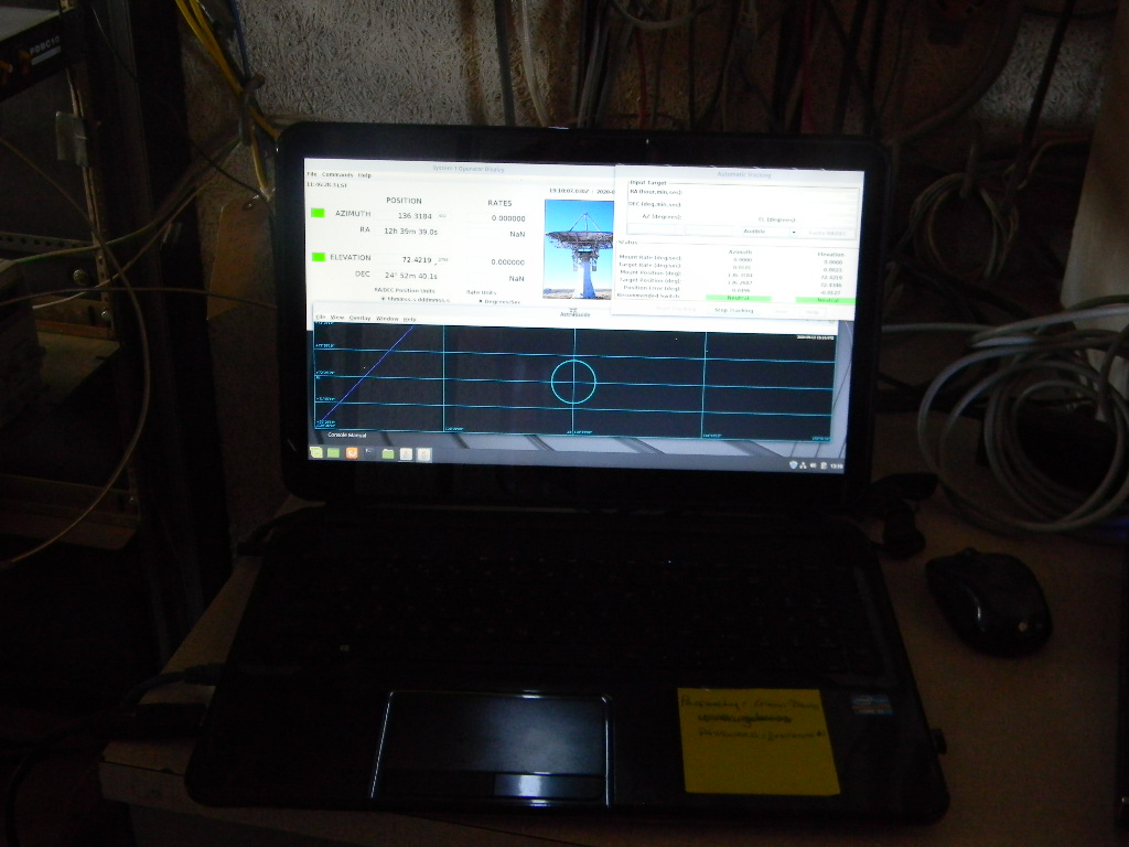
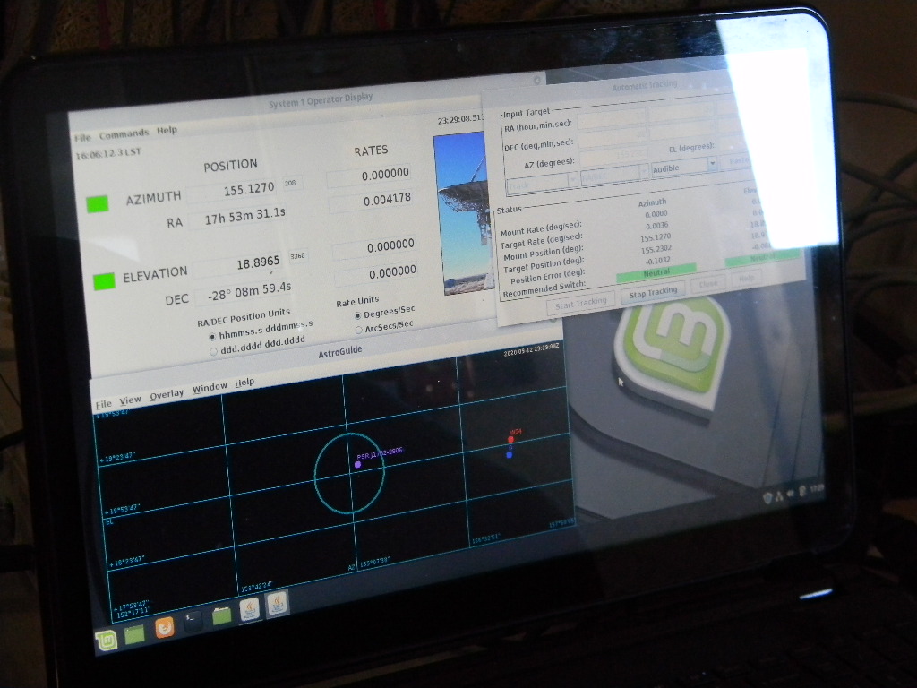
Rich and Bob are checking data for each next pulsar we attempt to observe. Besides the celestial coordinates, we need to know the expected energy flux. If the signal is weaker, we need to observe and track on the object for a longer period of time. We also need to know the expected pulse timing and several other parameters.We have up in our control room a framed photo of Jocelyn Bell Burnell, contributed by Bob Haggart. She discovered pulsars serendipitously while she was a graduate student at Cambridge University in 1967. Rich is assessing a good data set we just got. Here you can see the distinctive pulse timing spikes in the upper left. In the center white plot, you see two straight lines, representing the pulsed signal, across the spectrum of frequencies we observed (we observe across a bandwidth of 10 MHz). At the right, the software found a good analysis for the rate and change of rate of the pulses. The bottom plot slopes downward slightly to the right. That is showing us the dispersion of the signal, something we expect to see. As the pulsar radio signal travels through interstellar space, it has to go through dust and magnetic fields. The effect is that the longer the radio wavelength, the slower the signal will propagate through space. Therefore the longer wavelength signal will arrive slightly later than the shorter. This is an indirect measure of the distance to the pulsar. If the algorithm was just trying to make sense of random noise, we would not see this result in our data. (You can click this image to enlarge it.)This is a close-up of our SYSTEM 1 software display for pointing our dish antenna. The antenna now can be pointed manually or with several levels of automation.
The first accomplishment was to translate the actual azimuth and elevation pointing angles of the antenna through encoders with digital readouts. That azimuth and elevation angles were then correlated with the celestial coordinates at the given time. That required a good timing reference, as well as an accurate fix on our longitude and latitude. We now take care of that timing and position fix with GPS.
The upper part of the screen shows the direction the antenna is aimed at, in both azimuth and elevation angles, and the celestial coordinates of Right Ascension (RA) and Declination. There is more on the right side that was added later which I will discuss shortly.
The next development was to have a visual reference of the celestial sky, with its coordinate grid system and celestial objects we are interested, displayed on the computer, together with where the antenna is pointing. You see that display in the lower half of the screen. How wide a beam angle our antenna can see (like the field of view you see in an optical telescope) depends on the wavelength of the radio waves we are using. At a wavelength of 70 centimeters (about 400 MHz frequency), the beam width is about 2 degrees for our dish antenna. At wavelength of 21 centimeters (about 1420 MHz where the spectral line of neutral hydrogen is), the beam width is about 0.8 degrees. The software calculates the appropriate beam width and shows that as a circle on the display.
Within the last three months, our software team succeeded in creating a system that will now automatically point and keep tracking a celestial object or any other sky position. As part of this package, the software has a database of celestial objects we may be interested to look at, with their celestial coordinates. The database is updatable. If an object we want is in our database, it will appear on our sky coordinates display, we can point to it with our cursor, and the antenna will slew to point to it and then track it. We can also enter data manually. The software and hardware have safety stops, so that the antenna cannot be pointed below a certain limit above the horizon. And the antenna has azimuth limits, so that our cables to the antenna feed in the pedestal don’t wrap around with too many turns. The software also is programmed to avoid direct pointing towards the sun.
Because it makes the display much more user friendly, the display shows the visible stars and constellations as well. (You can click the image to enlarge it.)This screen is how we set our data parameters. And the display at lower left shows the signal coming in. The blue line is the data signal, across the bandwidth of 10 MHz, here centered at 420 MHz.
The green line shows the peak maximum of the signal over the course of the run. Earlier in the day we were seeing persistent radio signals, for us interference, at around 390, 406, 408, 410, and 432 MHz. We were concerned that one possible cause of problems with some of our data was the sun being close in angle to our pointing. We were never closer than 25 degrees from the sun. But we are wondering if the sun still might heat our preamplifiers at the feed focus of the antenna.The next set of photos are close-ups of the damage seen on the ham radio HF antennas. This is the tower with the 3-band Yagi. There is a slight tilt along the main boom.7 radials at the multi-band vertical antenna were also damaged. 5 severed at the lugs, which suggests metal fatigue from repeated moving in the wind. 2 were severed in their middles, which suggests some debris may have impacted those from the winds.Some of the fence damage by the bunker.The bunker ramp filled with tumbleweed again.Closeup of the 408 MHz feed and the feed mount at the focus of the 60 foot dish antenna. A closeup of the display we now use for pointing the dish antenna for astronomical observing. At the upper right, we can acquire the celestial coordinates from our database, or we can manually type in the needed data. The lower part of that window shows the actions the control system is executing, that is if it is slewing to an object, tracking, holding steady, or something else. The lower display shows the celestial sky, the coordinates, our antenna beam, as well as naked eye objects and constellations.The grain elevator in Haswell in the distance.